Support-vector machines, also known as SVMs, represent the cutting edge of statistical machine learning. They are typically used for classification problems, although they can be used for regression, too. SVMs often succeed at finding separation between classes when other models – that is, other learning algorithms – do not.
Scikit-learn makes building SVMs easy with classes such as SVC for classification models and SVR for regression models. You can use these classes without understanding how support-vector machines work, but you’ll get more out of them if you do understand how they work. It’s also important to know how to tune SVMs for individual datasets and how to prepare data before you train a model. At the end of this post, I’ll present an SVM that performs facial recognition. But first, let’s look behind the scenes and learn why SVMs are often the go-to mechanism for modeling real-world datasets.
How Support-Vector Machines Work
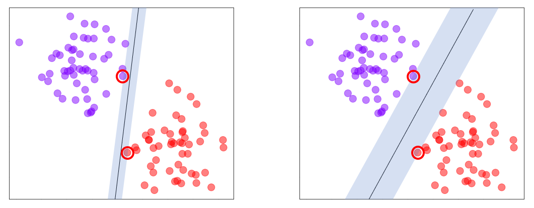
First, why are they called support-vector machines? The purpose of an SVM classifier is the same as any other classifier: to find a decision boundary that cleanly separates the classes. SVMs do this by finding a line in 2D space, a plane in 3D space, or a hyperplane in high-dimensional space that let them distinguish between different classes with the greatest margin of error possible. They do it by computing a decision boundary that provides the greatest margin along a line perpendicular to the boundary between the closest points, or support vectors, in the two classes. (SVMs perform binary classification only, but Scikit enables them to do multiclass classification using the techniques described in my previous post.) There’s an infinite number of lines you can draw to separate the two classes in the diagrams below, but the best line is the one that produces the widest margin. Support vectors are circled in red.
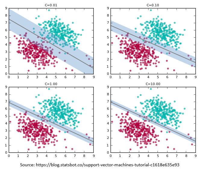
Of course, real-world data rarely lends itself to such clean separation. Overlap between classes inevitably prevents a perfect fit. To accommodate this, SVMs support a regularization parameter called C that can be adjusted to loosen or tighten the fit. Lower values of C produce a wider margin with more errors on either side of the decision boundary. Higher values yield a tighter fit to the training data with a correspondingly thinner margin and fewer errors. If C is too high, the model might not generalize well. The optimum value varies by dataset. Data scientists typically try different values of C to determine which one performs the best against test data.
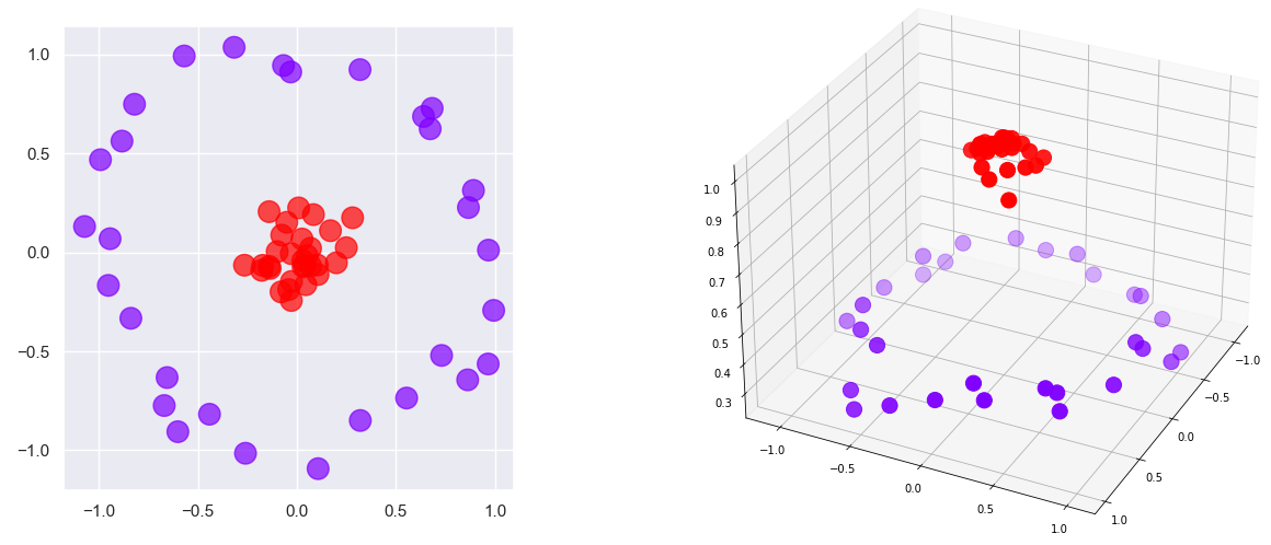
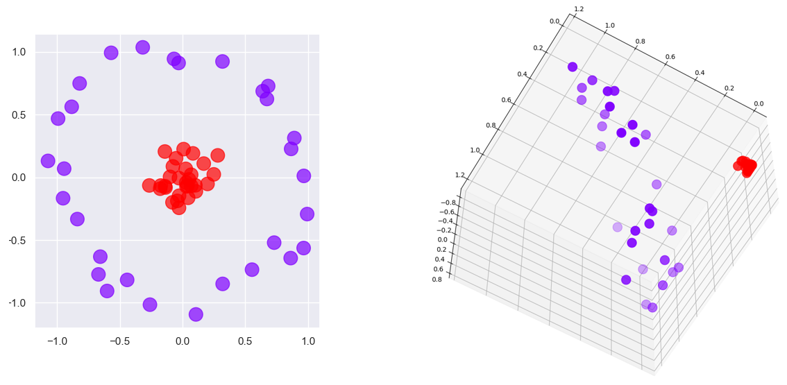
All of the above is true. But none of it explains why SVMs are so good at what they do. SVMs aren’t the only models that mathematically look for boundaries separating the classes. What makes SVMs special is kernels, some of which add dimensions to data to find boundaries that don’t exist at lower dimensions. Consider the figure at left below. You can’t draw a line that completely separates the red dots from the purple dots. But if you add a third dimension as shown on the right – a z dimension whose value is based on a point’s distance from the center – then you can slide a plane between the purples and the reds and achieve 100% separation. In this example, data that isn’t linearly separable in two dimensions is linearly separable in three dimensions. The principle at work here is Cover’s theorem, which states that data that isn’t linearly separable might be linearly separable if projected into a higher-dimensional space using a non-linear transform.
The kernel transformation used in this example, which “projects” 2-dimensional data to 3 dimensions by adding a z to every x and y, works well with this particular dataset. But for SVMs to be broadly useful, you need a kernel that isn’t tied to the shape of a specific dataset.
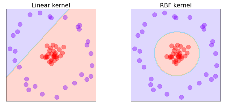
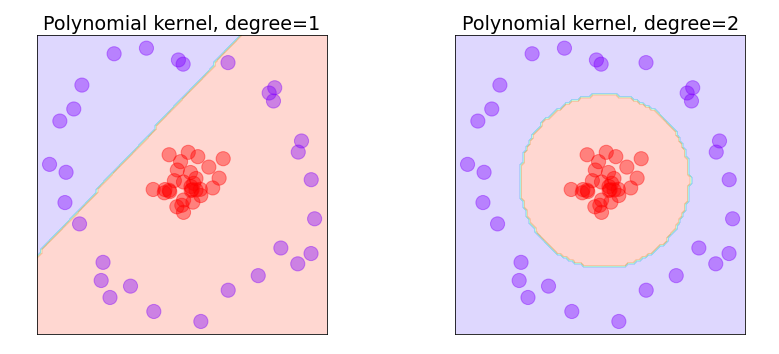
Scikit-learn has several general-purpose kernels built in, including the linear kernel, the RBF (short for radial basis function) kernel, and the polynomial kernel. The linear kernel doesn’t add dimensions. It works well with data that is linearly separable out of the box, but it doesn’t perform very well with data that isn’t. Applying it to the problem above produces the decision boundary on the left below. Applying the RBF kernel to the same data produces the decision boundary on the right. The RBF kernel projects the xs and ys into a higher-dimensional space and finds a hyperplane that cleanly separates the purples from the reds. When projected back to two dimensions, the decision boundary roughly forms a circle. Similar results can be achieved on this dataset with a properly tuned polynomial kernel, but generally speaking, the RBF kernel can find decision boundaries in non-linear data that the polynomial kernel cannot. That’s why RBF is the default kernel type in Scikit if you don’t specify otherwise.
A logical question to ask is what did the RBF kernel do? Did it add a z to every x and y? The short answer is no. It effectively projected the data points into a space with an infinite number of dimensions. The key word is effectively. Kernels use mathematical shortcuts called kernel tricks to measure the effect of adding new dimensions without actually computing values for them. This is where the math for SVMs gets hairy. Kernels are carefully designed to compute the dot product between two n-dimensional vectors in m-dimensional space (where m is greater than n and can even be infinite) without generating all those new dimensions, and ultimately, the dot products are all an SVM needs to compute a decision boundary. It’s the mathematical equivalent of having your cake and eating it, too, and it’s the secret sauce that makes SVMs awesome. SVMs can still take a relatively long time to train on large datasets, but one of the benefits of an SVM is that it tends to do better on smaller datasets with fewer rows or samples than other learning algorithms.
Kernel Tricks in Action
Want to see an example of how kernel tricks are used to compute dot products in high-dimensional spaces without computing values for the new dimensions? The following explanation is completely optional. But if you, like me, learn better from concrete examples, then you might find this section helpful.
Let’s start with the 2-dimensional circular dataset presented above, but this time, let’s project it into 3-dimensional space with the following equations:
![]()
In other words, we’ll compute x and y in 3-dimensional space by squaring x and y in 2-dimensional space, and we’ll add a z that’s the product of the original x and y and the square root of 2. Projecting the data this way produces a clean separation between purples and reds:
The efficacy of SVMs depends on their ability to compute the dot product of two vectors (or points, which can be treated as vectors) in higher-dimensional space without projecting them into that space – that is, using only the values in the original space. Let’s manufacture a couple of points to work with:
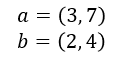
We can compute the dot product of these two points this way:
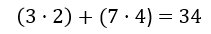
Of course, the dot product in two dimensions isn’t very helpful. An SVM needs the dot product of these points in 3D space. Let’s use the equations above to project a and b to 3D, and then compute the dot product of the result:
We now have the dot product of a pair of 2D points in 3D space, but we had to generate dimensions in 3D space in order to get it. Here’s where it gets interesting. The following function, or “kernel trick,” produces the same result using only the values in the original 2D space:
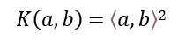
⟨a, b⟩ is simply the dot product of a and b, so ⟨a, b⟩2 is the square of the dot product of a and b. We already know how to compute the dot product of a and b. Therefore:

This agrees with the result we computed by explicitly projecting the points, but with no projection required. That’s the kernel trick in a nutshell. It saves time and memory when going from 2 dimensions to 3. Just imagine the savings when projecting to an infinite number of dimensions – which, you’ll recall, is exactly what the RBF kernel does.
The kernel trick used here wasn’t manufactured from thin air. It happens to be the one used by a degree-2 polynomial kernel. With Scikit, you can fit an SVM classifier with a degree-2 polynomial kernel to a dataset this way:
model = SVC(kernel='poly', degree=2)
model.fit(x, y)
If you apply this to the circular dataset above and plot the decision boundary, the result is almost identical to the one generated by the RBF kernel. Interestingly, a degree-1 polynomial kernel produces the same decision boundary as the linear kernel since a line is just a 1st degree polynomial:
Kernel tricks are special. Each one is designed to simulate a specific projection into higher dimensions. Scikit gives you a handful of kernels to work with, but there are others that Scikit doesn’t build in. You can extend Scikit with kernels of your own, but the ones that it provides are sufficient for the vast majority of use cases.
Hyperparameter Tuning
Going in, it’s difficult to know which of the built-in kernels will produce the most accurate model. It’s also difficult to know what the right value of C is – the value that provides the best balance between underfitting and overfitting the training data and yields the best results when the model is run with test data. For the RBF and polynomial kernels, there’s a third value called gamma that affects accuracy. And for polynomial kernels, the degree parameter impacts the model’s ability to learn from the training data.
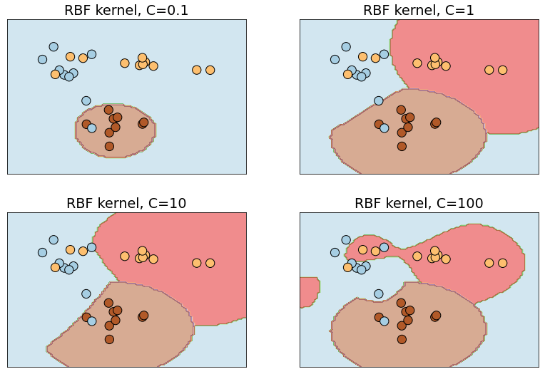
The C parameter controls how aggressively the model fits to the training data. The higher the value, the tighter the fit and the higher the risk of overfitting. The diagram below shows how the RBF kernel fits a model to a set of training data containing three classes with different values of C. The default is C=1 in Scikit, but you can specify a different value to adjust the fit. You can see the danger of overfitting in the diagram at lower right. A point that lies to the extreme right would be classified as a blue, even though it probably belongs to the yellow or brown class. Underfitting is a problem, too. In the example at upper left, virtually any data point that isn’t a brown will be classified as a blue.
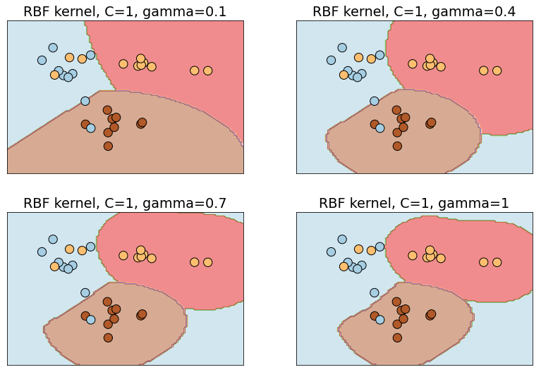
An SVM that uses the RBF kernel isn’t properly tuned until you have the right value for gamma, too. gamma controls how far the influence of a single data point reaches in computing decision boundaries. Lower values use more points and produce smoother decision boundaries; higher values involve fewer points and fit more tightly to the training data. This is illustrated below, where increasing gamma while holding C constant closes the decision boundary more tightly around clusters of classes. gamma can be any non-zero positive value, but values between 0 and 1 are the most common. Rather than hard-code a default value for gamma, Scikit picks a default value algorithmically if you don’t specify one.
In practice, data scientists experiment with different kernels and different parameter values to find the combination that produces the most accurate model, a process known as hyperparameter tuning. The usefulness of hyperparameter tuning isn’t unique to SVMs, but you can almost always make an SVM more accurate by finding the optimum combination of kernel type, C, and gamma (and for polynomial kernels, degree).
To aid in the process of hyperparameter tuning, Scikit provides a family of optimizers that includes GridSearchCV, which tries all combinations of a specified set of parameter values with built-in cross-validation to determine which combination produces the most accurate model. These optimizers prevent you from having to write code to do a brute-force search using all the unique combinations of parameter values. To be clear, they do brute-force searches themselves by training the model multiple times, each time with a different combination of values. At the end, you can retrieve the most accurate model from the best_estimator_ attribute, the parameter values that produced the most accurate model from the best_params_ attribute, and the best score from the best_score_ attribute.
Here’s an example that uses Scikit’s SVC class to implement an SVM classifier. For starters, you can create an SVM classifier that uses default parameter values and fit it to a dataset with two lines of code:
model = SVC()
model.fit(x, y)
This uses the RBF kernel with C=1. You can specify the kernel type and values for C and gamma this way:
model = SVC(kernel='poly', C=10, gamma=0.1)
model.fit(x, y)
Suppose you wanted to try two different kernels and five values each for C and gamma to see which combination produces the best results. Rather than write a nested for loop, you could do this instead:
model = SVC()

grid = {
    'C': [0.01, 0.1, 1, 10, 100],
    'gamma': [0.01, 0.25, 0.5, 0.75, 1.0],
    'kernel': ['rbf', 'poly']
}

grid_search = GridSearchCV(estimator=model, param_grid=grid, cv=5, verbose=2)
grid_search.fit(x, y) # Train the model with different parameter combinations
The call to fit won’t return for a while. It trains the model 250 times since there are 50 different combinations of kernel, C, and gamma, and cv=5 says uses 5-fold cross-validation to assess the results. Once training is complete, you can get the best model this way:
best_model = grid_search.best_estimator_
It is not uncommon to run a search regimen such as this one multiple times – the first time with course parameter values, and each time thereafter with narrower ranges of values centered around the values obtained from best_params_. More training time up front is the price you pay for an accurate model. To reiterate, you can almost always make an SVM more accurate by finding the optimum combination of parameters. And for better or worse, brute force is the most effective way to identify the best combination.
Data Standardization
In my post on regression algorithms, I noted that some learning algorithms work better with normalized data. Unnormalized data contains columns of numbers with vastly different ranges – for example, values from 0 to 1 in one column and 0 to 1,000,000 in another. Scikit’s MinMaxScaler class normalizes data by proportionally reducing the values in each column to values from 0.0 to 1.0. But that’s not enough for a typical SVM.
SVMs tend to be sensitive to unnormalized data. Moreover, they like data that is normalized to unit variance using a technique called standardization or Z-score normalization. Unit variance is achieved by doing the following to each column in a dataset:
- Compute the mean and standard deviation of all the values in the column
- Subtract the mean from each value in the column
- Divide each value in the column by the standard deviation
This is precisely the transform that Scikit’s StandardScaler class performs on a dataset. Normalizing a dataset to have unit variance is as simple as this:
scaler = StandardScaler()
x = scaler.fit_transform(x)
The values in the original dataset may vary wildly from one column to the next, but the transformed dataset will contain columns of numbers centered around 0 with ranges that are proportional to each column’s standard deviation. SVMs typically perform better when trained with standardized data, even if all the columns have similar ranges. (The same is true of neural networks, by the way.) The classic case in which columns having similar ranges is image data, where each column holds pixel values from 0 to 255. There are exceptions, but it is usually a mistake to throw a bunch of data at an SVM without understanding the shape of the data – specifically, whether it has unit variance.
Pipelining
If you standardize the values used to train a machine-learning model, you must apply the same transform to values input to the model’s predict method. In other words, if you train a model this way:
model = SVC()
scaler = StandardScaler()
x = scaler.fit_transform(x)
model.fit(x, y)
Then you make predictions with it this way:
input = [0, 1, 2, 3, 4]
model.predict([scaler.transform([input])
Otherwise, you’ll get non-sensical predictions.
To simplify your code and make it harder to forget to transform training data and prediction data the same way, Scikit offers the make_pipeline function. make_pipeline lets you combine predictive models – what Scikit calls estimators, or instances of classes such as SVC – with transforms applied to data input to those models. Here’s how you use make_pipeline to ensure that any data input to the model is transformed the same way with StandardScaler:
# Train the model
pipe = make_pipeline(StandardScaler(), SVC())
pipe.fit(x, y)

# Make a prediction with the model
input = [0, 1, 2, 3, 4]
pipe.predict([input])
Now data used to train the model has StandardScaler applied to it, and data input to make predictions is transformed with the same StandardScaler.
What if you wanted to use GridSearchCV to find the optimum set of parameters for a pipeline that combines a data transform and estimator? It’s not hard, but there’s a trick you need to know about. It involves using class names prefaced with double underscores in the param_grid dictionary passed to GridSearchCV. Here’s an example:
pipe = make_pipeline(StandardScaler(), SVC())

grid = {
    'svc__C': [0.01, 0.1, 1, 10, 100],
    'svc__gamma': [0.01, 0.25, 0.5, 0.75, 1.0],
    'svc__kernel': ['rbf', 'poly']
}

grid_search = GridSearchCV(estimator=pipe, param_grid=grid, cv=5, verbose=2)
grid_search.fit(x, y) # Train the model with different parameter combinations
This example trains the model 250 times to find the best combination of kernel, C, and gamma for the SVC instance in the pipeline. Note the svc__ nomenclature, which maps to the SVC instance passed to the make_pipeline function.
Train an SVM to Perform Facial Recognition
Facial recognition is often accomplished with neural networks, but support-vector machines can do a credible job, too. Let’s demonstrate by building a Jupyter notebook that recognizes faces. The dataset we’ll use is the Labeled Faces in the Wild (LFW) dataset, which contains more than 13,000 facial images of famous people collected from around the Web and is built into Scikit as a sample dataset. Of the more than 5,000 people represented in the dataset, 1,680 have two or more facial images, while only five have 100 or more. We’ll set the minimum number of faces per person to 100, which means that five sets of faces corresponding to five famous people will be imported. Each facial image is labeled with the name of the person that the face belongs to.
Start by creating a new notebook and using the following statements to load the dataset:
import numpy as np
import pandas as pd
from sklearn.datasets import fetch_lfw_people

faces = fetch_lfw_people(min_faces_per_person=100)
print(faces.target_names)
print(faces.images.shape)
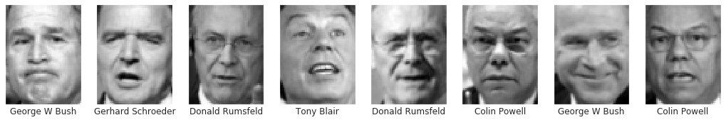
In total, 1,140 facial images were loaded. Each image measures 62 by 47 pixels for a total of 2,914 pixels per image. That means we’re working with a dataset containing 2,914 feature columns. Use the following code to show the first 24 images in the dataset and the people to whom the faces belong:
%matplotlib inline
import matplotlib.pyplot as plt

fig, ax = plt.subplots(3, 8, figsize=(18, 10))
for i, axi in enumerate(ax.flat):
    axi.imshow(faces.images[i], cmap='gist_gray')
    axi.set(xticks=[], yticks=[], xlabel=faces.target_names[faces.target[i]])
Check the balance in the dataset by generating a histogram showing how many facial images were imported for each person:
from collections import Counter
counts = Counter(faces.target)
names = {}

for key in counts.keys():
    names[faces.target_names[key]] = counts[key]

df = pd.DataFrame.from_dict(names, orient='index')
df.plot(kind='bar')
There are far more images of George W. Bush than of anyone else in the dataset. Classification models are best trained with balanced datasets. Use the following code to reduce the dataset to 100 images of each person:
mask = np.zeros(faces.target.shape, dtype=np.bool)

for target in np.unique(faces.target):
    mask[np.where(faces.target == target)[0][:100]] = 1

x = faces.data[mask]
y = faces.target[mask]
x.shape
x contains 500 facial images, and y contains the labels that go with them: 0 for Colin Powell, 1 for Donald Rumsfeld, and so on. Now let’s see if an SVM can make sense of the data. We’ll train three different models: one that uses a linear kernel, one that uses a polynomial kernel, and one that uses an RBF kernel. In each case, we’ll use GridSearchCV to optimize hyperparameters. Start with a linear model:
from sklearn.svm import SVC
from sklearn.model_selection import GridSearchCV

svc = SVC(kernel='linear')

grid = {
    'C': [0.1, 1, 10, 100]
}

grid_search = GridSearchCV(estimator=svc, param_grid=grid, cv=5, verbose=2)
grid_search.fit(x, y) # Train the model with different parameters
grid_search.best_score_
This model achieves a cross-validated accuracy of 84.4%. It’s possible that accuracy can be improved by standardizing the image data. Run the same grid search again, but this time use StandardScaler to apply unit variance to all the pixel values:
from sklearn.pipeline import make_pipeline
from sklearn.preprocessing import StandardScaler

scaler = StandardScaler()
svc = SVC(kernel='linear')
pipe = make_pipeline(scaler, svc)

grid = {
    'svc__C': [0.1, 1, 10, 100]
}

grid_search = GridSearchCV(estimator=pipe, param_grid=grid, cv=5, verbose=2)
grid_search.fit(x, y)
grid_search.best_score_
Standardizing the data produced an incremental improvement in accuracy. What value of C produced that accuracy?
grid_search.best_params_
Is it possible that a polynomial kernel could outperform a linear kernel? There’s an easy way to find out. Note the introduction of the gamma and degree parameters to the parameter grid. These parameters, along with C, can greatly influence a polynomial kernel’s ability to fit to the training data.
scaler = StandardScaler()
svc = SVC(kernel='poly')
pipe = make_pipeline(scaler, svc)

grid = {
    'svc__C': [0.1, 1, 10, 100],
    'svc__gamma': [0.01, 0.25, 0.5, 0.75, 1],
    'svc__degree': [1, 2, 3, 4, 5]
}

grid_search = GridSearchCV(estimator=pipe, param_grid=grid, cv=5, verbose=2)
grid_search.fit(x, y) # Train the model with different parameter combinations
grid_search.best_score_
The polynomial kernel achieved the same accuracy as the linear kernel. What parameter values led to this result?
grid_search.best_params_
best_params_ reveals that the optimum value of degree was 1, which means the polynomial kernel acted like a linear kernel. It’s not surprising, then, that it achieved the same accuracy. Could an RBF kernel do better?
scaler = StandardScaler()
svc = SVC(kernel='rbf')
pipe = make_pipeline(scaler, svc)

grid = {
    'svc__C': [0.1, 1, 10, 100],
    'svc__gamma': [0.01, 0.25, 0.5, 0.75, 1.0]
}

grid_search = GridSearchCV(estimator=pipe, param_grid=grid, cv=5, verbose=2)
grid_search.fit(x, y)
grid_search.best_score_
The RBF kernel didn’t perform as well as the linear and polynomial kernels. There’s a lesson here. The RBF kernel often fits to non-linear data better than other kernels, but it doesn’t always fit better. That’s why the best strategy with an SVM is to try different kernels with different parameter values. The best combination will vary from dataset to dataset. For the LFW dataset, it seems that a linear kernel is best. That’s convenient, because the linear kernel is the fastest of all the kernels that Scikit provides.
Confusion matrices are a great way to visualize a model’s accuracy. Let’s split the dataset, train an optimized linear model with 80% of the images, test it with the remaining 20%, and show the results in a confusion matrix.
The first step is to split the dataset. Note the stratify=y parameter, which ensures that the training dataset and the test dataset have the same proportion of samples of each class as the original dataset. In this example, the training dataset will contain 20 samples of each of the five people.
from sklearn.model_selection import train_test_split

x_train, x_test, y_train, y_test = train_test_split(x, y, train_size=0.8, stratify=y, random_state=0)
Now train a linear SVM with the optimum C value revealed by the grid search:
scaler = StandardScaler()
svc = SVC(kernel='linear', C=0.1)
pipe = make_pipeline(scaler, svc)
pipe.fit(x_train, y_train)
Cross-validate the model to confirm that it’s as accurate when trained with 80% of the dataset as it was when it was trained with the entire dataset:
from sklearn.model_selection import cross_val_score

cross_val_score(pipe, x, y, cv=5).mean()
Use a confusion matrix to see how the model performs against the test data:
from sklearn.metrics import plot_confusion_matrix

plot_confusion_matrix(pipe, x_test, y_test, display_labels=faces.target_names, cmap='Blues', xticks_rotation='vertical')
The model correctly identified Colin Powell 19 times out of 20, Donald Rumsfeld 20 times out of 20, and so on. That’s not bad. And it’s a great example of support-vector machines at work. It would be challenging, perhaps impossible, to do this well using more conventional learning algorithms such as logistic regression.
Wrapping Up
You can download a Jupyter notebook containing the facial-recognition example in this post from the machine-learning repo that I maintain on GitHub. Feel free to check out the other notebooks in the repo while you’re at it. Also be sure to check back from time to time because I am constantly uploading new samples and updating existing ones.
One nuance to be aware of regarding the SVC class is that it doesn’t compute probabilities by default. If you want to call predict_proba on an SVC instance, you must set probability to True when creating the instance:
model = SVC(probability=True)
The model will train slower, but you’ll be able to retrieve probabilities as well as predictions.
Finally, if you’d like to learn more about SVMs, kernels, and kernel tricks, I highly recommend reading Support Vector Machine (SVM) Tutorial by Abhishek Ghose. It’s wonderfully written and is one of the best articles I’ve seen for building an intuitive understanding of how SVMs work.