My previous post introduced a machine-learning model that used logistic regression to predict whether text input to it expresses positive or negative sentiment. We used the probability that the text expresses positive sentiment as a sentiment score, and saw that expressions such as “The long lines and poor customer service really turned me off” score close to 0.0, while expressions such as “The food was great and the service was excellent” score close to 1.0. In this post, we’ll build a binary-classification model that classifies e-mails as spam or not spam. And we’ll use a learning algorithm called Naïve Bayes to fit the model to the training data.
It’s no coincidence that modern spam filters are incredibly good at identifying spam. Virtually all of them rely on machine learning. Such models are difficult to implement algorithmically, because an algorithm that uses keywords such as “credit” and “score” to determine whether an e-mail is spam is easily fooled. Machine learning, by contrast, looks at a body of e-mails and uses what it learns to classify the next e-mail. Such models often achieve more than 99% accuracy. And they get smarter over time as they’re trained with more and more e-mails.
Naïve Bayes
Naïve Bayes is a classification algorithm based on Bayes theorem, which provides a means for calculating conditional probabilities. Mathematically, Bayes theorem is stated this way:
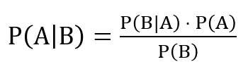
This says the probability that A is true if B is true is equal to the probability that B is true if A is true multiplied by the probability that A is true divided by the probability that B is true. That’s a mouthful, and while accurate, it doesn’t explain why Naïve Bayes is so useful for classifying text – or how you apply the equation to a bunch of e-mails in order to determine which ones are spam.
It turns out that if you make some simple (naïve) assumptions – that the order of the words in an e-mail doesn’t matter, and that every word has equal weight – you can write the equation this way for text classification:

In plain English, the probability that a message is spam is proportional to the product of:
- The probability that any message in the dataset is spam (P(S))
- The probability that each word in the message appears in a spam message (P(word|S))
P(S) can be calculated easily enough; it’s just the fraction of the messages in the dataset that are spam messages. If you train a machine-learning model with 1,000 messages and 500 of them are spam, then P(S) = 0.5. For a given word, P(word|S) is simply the number of times the word appears in spam messages divided by the number of words in all the spam messages. The entire problem reduces to word counts. What’s really cool is that you can do a similar calculation to compute the probability that the message is not spam, and then use the higher of the two probabilities to make a prediction.
Here’s an example involving four sample e-mails. The e-mails are:
| Text | Spam |
| Raise your credit score in minutes | 1 |
| Here are the minutes from yesterday’s meeting | 0 |
| Meeting tomorrow to review yesterday’s scores | 0 |
| Score tomorrow’s meds at yesterday’s prices | 1 |
If you remove stop words, convert characters to lowercase, and stem the words such that “tomorrow’s” becomes “tomorrow,” you’re left with this:
| Text | Spam |
| raise credit score minute | 1 |
| minute yesterday meeting | 0 |
| meeting tomorrow review yesterday score | 0 |
| score tomorrow med yesterday price | 1 |
Because two of the four messages are spam and two are not, the probability that any message is spam (P(S)) is 0.5. The same goes for the probability that any message is not spam (P(N) = 0.5). In addition, the spam messages contain a total of 9 words, while the non-spam messages contain a total of 8.
The next step is to build the table of word frequencies below. Take the word “yesterday” as an example. It appears once in a message that’s labeled as spam, so P(yesterday|S) is 1/9, or 0.111. It appears twice in non-spam messages, so P(yesterday|N) is 2/8, or 0.250.
| Word | P(word|S) | P(word|N) |
| raise | 1/9 = 0.111 | 0/8 = 0.000 |
| credit | 1/9 = 0.111 | 0/8 = 0.000 |
| score | 2/9 = 0.222 | 1/8 = 0.125 |
| minute | 1/9 = 0.111 | 1/8 = 0.125 |
| yesterday | 1/9 = 0.111 | 2/8 = 0.250 |
| meeting | 0/9 = 0.000 | 2/8 = 0.250 |
| tomorrow | 1/9 = 0.111 | 1/8 = 0.125 |
| review | 0/9 = 0.000 | 1/8 = 0.125 |
| med | 1/9 = 0.111 | 0/8 = 0.000 |
| price | 1/9 = 0.111 | 0/8 = 0.000 |
This works up to a point, but the zeros in the table are a problem. Let’s say you want to determine whether “Scores must be reviewed by tomorrow” is spam. Removing stop words leaves you with “score review tomorrow.” You can compute the probability that the message is spam this way:
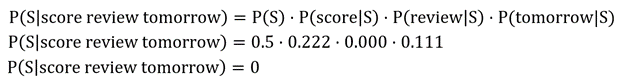
The result is 0 because “review” doesn’t appear in a spam message, and 0 times anything is 0. The algorithm simply can’t assign a spam probability to “Scores must be reviewed by tomorrow.”
A common way to resolve this is to apply Laplace smoothing, also known as additive smoothing. Typically, this involves adding 1 to each numerator and the number of unique words in the dataset (in this case, 10) to each denominator. Now, P(review|S) evaluates to (0 + 1) / (9 + 10), which equals 0.053. It’s not much, but it’s better than nothing (literally). Here are the word frequencies again, this time revised to use Laplace smoothing:
| Word | P(word|S) | P(word|N) |
| raise | (1 + 1) / (9 + 10) = 0.105 | (0 + 1) / (8 + 10) = 0.056 |
| credit | (1 + 1) / (9 + 10) = 0.105 | (0 + 1) / (8 + 10) = 0.056 |
| score | (2 + 1) / (9 + 10) = 0.158 | (1 + 1) / (8 + 10) = 0.111 |
| minute | (1 + 1) / (9 + 10) = 0.105 | (1 + 1) / (8 + 10) = 0.111 |
| yesterday | (1 + 1) / (9 + 10) = 0.105 | (2 + 1) / (8 + 10) = 0.167 |
| meeting | (0 + 1) / (9 + 10) = 0.053 | (2 + 1) / (8 + 10) = 0.167 |
| tomorrow | (1 + 1) / (9 + 10) = 0.105 | (1 + 1) / (8 + 10) = 0.111 |
| review | (0 + 1) / (9 + 10) = 0.053 | (1 + 1) / (8 + 10) = 0.111 |
| med | (1 + 1) / (9 + 10) = 0.105 | (0 + 1) / (8 + 10) = 0.056 |
| price | (1 + 1) / (9 + 10) = 0.105 | (0 + 1) / (8 + 10) = 0.056 |
Now you can determine whether “Scores must be reviewed by tomorrow” is spam by performing two simple calculations:
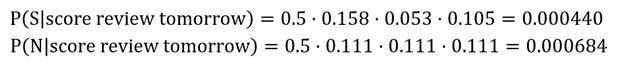
By this measure, “Scores must be reviewed by tomorrow” is likely not to be spam. The probabilities are relative, but you could normalize them and conclude there’s a 40% chance the message is spam and a 60% chance it’s not based on the e-mails the model was trained with.
Fortunately, you don’t have to do these computations by hand. Scikit-learn provides several classes to help out, including the MultinomialNB class, which works great with tables of word counts produced by CountVectorizer. CountVectorizer was introduced in the previous post in this series and it includes the ability to remove stop words as well as convert text to lowercase and consider n-grams (groups of n consecutive words) rather than just individual words.
Train a Spam Classifier
Let’s put MultinomialDB and CountVectorizer to work building a model that examines an e-mail and tells us whether that e-mail is spam, as well as the probability that it’s spam.
There are several spam-classification datasets available in the public domain. Each contains a collection of e-mails with samples labeled with 1s for spam and 0s for not spam. We’ll use a relatively small dataset containing 1,000 samples. Begin by downloading the dataset and copying it into your notebooks’ “Data” subdirectory. Then use the following code to load the data and display the first five rows:
import pandas as pd

df = pd.read_csv('Data/ham-spam.csv')
df.head()
Now check for duplicate rows in the dataset:
df.groupby('IsSpam').describe()
The dataset contains one duplicate row. Let’s remove it and check for balance:
df = df.drop_duplicates()
df.groupby('IsSpam').describe()
The dataset now contains 499 samples that are not spam, and 500 that are. The next step is to use CountVectorizer to vectorize the e-mails. For good measure, we’ll allow CountVectorizer to consider word pairs as well as individual words and remove stop words using Scikit’s built-in dictionary of more than 300 English stop words:
from sklearn.feature_extraction.text import CountVectorizer

vectorizer = CountVectorizer(ngram_range=(1, 2), stop_words='english')
x = vectorizer.fit_transform(df['Text'])
y = df['IsSpam']
Split the dataset so that 80% can be used for training and 20% for testing:
from sklearn.model_selection import train_test_split

x_train, x_test, y_train, y_test = train_test_split(x, y, test_size=0.2, random_state=0)
The next step is to train a Naïve Bayes classifier. We’ll use Scikit’s MultinomialDB class, which is ideal for datasets vectorized by CountVectorizer:
from sklearn.naive_bayes import MultinomialNB

model = MultinomialNB()
model.fit(x_train, y_train)
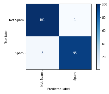
Validate the trained model with the 20% of the dataset set aside for testing and show a confusion matrix:
%matplotlib inline
from sklearn.metrics import plot_confusion_matrix

plot_confusion_matrix(model, x_test, y_test, display_labels=['Not Spam', 'Spam'], cmap='Blues', xticks_rotation='vertical')
The model correctly identified 101 of 102 legitimate e-mails as not spam, and 95 of 98 spam e-mails as spam.
Use the score method to get a rough measure of the model’s accuracy:
model.score(x_test, y_test)
Now compute the area under the Receiver Operating Characteristic (ROC) curve for a better measure of the model’s accuracy:
from sklearn.metrics import roc_auc_score

probabilities = model.predict_proba(x_test)
roc_auc_score(y_test, probabilities[:, 1])
The results are encouraging. Trained with just 999 samples, the model is more than 99.9% accurate at classifying e-mails as spam or not spam. Let’s see how the model classifies a few e-mails that it hasn’t seen before, starting with one that isn’t spam. The model’s predict method predicts a class: 0 for not spam, or 1 for spam.
message = vectorizer.transform(['Can you attend a code review on Tuesday? Need to make sure the logic is rock solid.'])
model.predict(message)[0]
The model says this message is not spam, but what’s the probability that it’s not spam? You can get that from predict_proba, which returns an array containing two values: the probability that the predicted class is 0, and the probability that the predicted class is 1, in that order.
model.predict_proba(message)[0][0]
Now test the model with a spam message:
message = vectorizer.transform(['Why pay more for expensive meds when you can order them online and save $$$?'])
model.predict(message)[0]
What is the probability that the message is not spam?
model.predict_proba(message)[0][0]
What is the probability that the message is spam?
model.predict_proba(message)[0][1]
Observe that predict and predict_proba accept an array of inputs. Based on that, could you classify an entire batch of e-mails with one call to predict or predict_proba? How would you get the results for each e-mail?
Get the Code
You can download a Jupyter notebook containing this example from the machine-learning repo that I maintain on GitHub. Feel free to check out the other notebooks in the repo while you’re at it. Also be sure to check back from time to time because I am constantly uploading new samples and updating existing ones.