When you build a machine-learning model, the first and most important decision you make is what learning algorithm to use to fit the model to the training data. In my previous post, I introduced some of the most widely used learning algorithms for regression models: linear regression, decision trees, random forests, gradient-boosting machines (GBMs), and support-vector machines (SVMs). In this post, we’ll put these algorithms to work building a regression model that predicts taxi fares from data published by the New York City Taxi & Limousine Commission.
Before we start slinging code, there is an important topic that needs to be addressed. That topic is scoring. As you know, you need one set of data with which to train a model, and another set for testing it. Testing (scoring) quantifies how accurate the model is at making predictions. It is incredibly important to test a model with a dataset other than the one it was trained with because it will probably learn the training data reasonably well, but that doesn’t mean it will generalize well – that is, make accurate predictions. And if you don’t score a model, you don’t know how accurate it is.
Earlier, we used Scikit’s train_test_split function to split a dataset into a training dataset and a testing dataset. But when you split data this way, you can’t necessarily trust the score returned by the model’s score method. And what does the score mean, anyway? The answer is different for regression models and classification models, and while there are a handful of ways to score regression models, there are many ways to score classification models. Let’s take a moment to understand the number that score returns for a regression model, and what you can do to have more faith in that number.
Scoring Regression Models
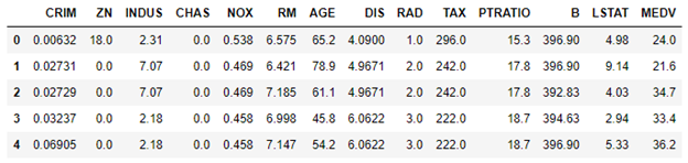
To demonstrate why you need to be somewhat skeptical of the number returned when you call score, try a simple experiment. Start by using the following code to load the Boston housing dataset, which is one of several sample datasets included in Scikit:
import pandas as pd
from sklearn.datasets import load_boston

boston = load_boston()
df = pd.DataFrame(boston.data, columns=boston.feature_names)
df['MEDV'] = boston.target
df.head()
The dataset contains several cryptically named columns such as CRIM (per capita crime rate), ZN (proportion of residential land zoned for lots larger than 25,000 square feet), and MEDV (median value of owner-occupied homes in thousands of dollars). The meanings aren’t important for now. What is important is that we are going to build a model that uses the 13 feature columns to predict MEDV values.
Use the code below to split the data 80/20, train a linear-regression model with 80% of the data to predict the price of a house, and score the model with the 20% of the data split off for testing:
from sklearn.linear_model import LinearRegression
from sklearn.model_selection import train_test_split

x_train, x_test, y_train, y_test = train_test_split(boston.data, boston.target, test_size=0.2, random_state=0)

model = LinearRegression()
model.fit(x_train, y_train)
model.score(x_test, y_test)
score returns 0.5892, which ostensibly indicates that the model was about 59% accurate using the features in the test data to make predictions and comparing the predictions to values in the MEDV column. So far, so good.
Now change the random_state value passed to train_test_split from 0 to 2 and run the code again:
x_train, x_test, y_train, y_test = train_test_split(boston.data, boston.target, test_size=0.2, random_state=2)

model = LinearRegression()
model.fit(x_train, y_train)
model.score(x_test, y_test)
This time, score returns 0.7789. So which is it? Is the model 59% accurate at making predictions or 78% accurate? Why did score return two different values?
When train_test_split splits a dataset, it randomly selects rows for the training dataset and the testing dataset. The random_state parameter seeds the random-number generator used to make the random selections. Seed it with 0, and the data gets split one way. Seed it with 2, and it gets split another way. By specifying two different seed values, you train the model with two different datasets and test it with two different datasets, too. Sure, there is overlap between them. But the fact remains that the number you seed train_test_split’s random-number generator with affects the outcome. The differences tend to be more pronounced with smaller datasets, but they show up with larger datasets, too.
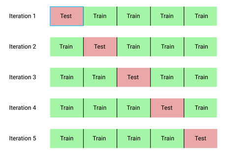
The solution is cross-validation. To cross-validate a model, you partition the dataset into folds as pictured below. Using five folds is common, but you can use any number of folds you like. Then you train the model five times – once for each fold – using a different 80% of the dataset for training and a different 20% for testing each time, and average the scores to generate a cross-validated score. That score is more reliable than the score returned by score because it is less sensitive to how the data is split. This process is known as k-fold cross validation.
The downside to cross-validation is that it takes longer. With 5-fold cross-validation, you’re training the model five times. If the model trains in a few seconds, it’s no big deal. But some of today’s state-of-the-art models take weeks to train on datasets containing millions of images.
You don’t need to cross-validate if you’re given separate datasets for training and testing. Remember that the main justification for cross-validation is to make sure splits performed by train_test_split don’t affect the outcome.
You could write the code to do cross-validation yourself, but you don’t have to because Scikit does it for you. Cross-validating a model usually requires just one line of code:
from sklearn.model_selection import cross_val_score

cross_val_score(model, boston.data, boston.target, cv=5).mean()
In some cases (the Boston housing dataset is one of them), you need to shuffle the dataset before dividing it into folds. That requires one extra line of code. Use the code below to generate a cross-validated score for your regression model. How does the score compare to the scores generated by the model’s score method?
from sklearn.model_selection import KFold
from sklearn.model_selection import cross_val_score

k_fold = KFold(shuffle=True, random_state=0)
cross_val_score(model, boston.data, boston.target, cv=k_fold).mean()
If in doubt, it never hurts to shuffle the data prior to using it for cross-validation.
Which begs the question: precisely what does the value returned when you score or cross-validate a model represent? For a regression model, it’s the coefficient of determination, also known as R-squared or simply R2. The coefficient of determination is usually a value from 0 to 1 (“usually” because there are multiple definitions of coefficient of determination) which quantifies the variance in the output that can be explained by the variables in the input. A simple way to think of it is that an R2 score of 0.8 means that the model should, on average, be about 80% accurate in making predictions, or get the answer right within 20%. The higher the R2 score, the more accurate the model. There are other ways to measure the accuracy of a regression model, including mean squared error (MSE) and mean absolute error (MAE). Those numbers are only meaningful in the context of the range of output values, whereas R2 gives you one simple number that is independent of range. You can read more about regression metrics and methods for retrieving them in the Scikit documentation.
The value returned by a model’s score method is completely different for a classification model. I will address the various ways to quantify the accuracy of classification models in a future post.
Build a Regression Model to Predict Taxi Fares
Imagine that you work for a taxi company, and one of your customers’ biggest complaints is that they don’t know how much a ride will cost until it’s over. That’s because distance isn’t the only variable that determines a fare amount. You decide to do something about it by building a mobile app that customers can use when they climb into a taxi to estimate what the fare will be. To provide the smarts for the app, you intend to use the massive amounts of fare data the company has collected over the years to build a machine-learning model.

Regression models predict numeric outcomes such as the price of a car, the age of a person in a picture, or the cost of a taxi ride. Let’s train a regression model to predict a fare amount given the time of day, the day of the week, and the pickup and drop-off locations.
Start by downloading the CSV file containing the dataset and copying it into the “Data” subdirectory where your Jupyter notebooks are hosted. Then use the code below to load the dataset into a notebook. The dataset contains about 55,000 rows and is a subset of a much larger dataset that was recently used in Kaggle’s New York City Taxi Fare Prediction competition. The data requires a fair amount of prep work before it’s of any use at all — something that is not uncommon in machine learning. Data scientists often find that collecting and preparing data accounts for 90% or more of their time.
import pandas as pd
import matplotlib.pyplot as plt
%matplotlib inline
import seaborn as sns
sns.set()

df = pd.read_csv('Data/taxi-fares.csv')
df.head()
Here’s the output from the code:
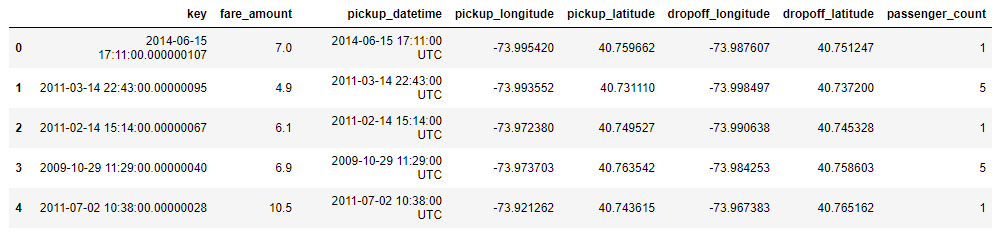
Each row represents a taxi ride and contains information such as the fare amount, the pickup and drop-off locations (expressed as latitudes and longitudes), and the passenger count. It’s the fare amount that we’ll try to predict. Use the following code to draw a histogram showing how many rows contain a passenger count of 1, how many contain a passenger count of 2, and so on:
sns.countplot(x=df['passenger_count'])
Here is the output:
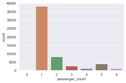
Most of the rows in the dataset have a passenger count of 1. Since we’re only interested in predicting the fare amount for single passengers, use the code below to remove all rows with multiple passengers and remove the “key” column from the dataset since that column isn’t needed – in other words, it’s not one of the features that we will try to predict on:
df = df[df['passenger_count'] == 1]
df = df.drop(['key', 'passenger_count'], axis=1)
df.head()
That leaves 38,233 rows in the dataset, which you can see for yourself with the following statement:
df.shape
Now use Pandas’s corr method to find out how much influence input variables such as latitude and longitude have on the values in the “fare_amount” column:
corr_matrix = df.corr()
corr_matrix['fare_amount'].sort_values(ascending=False)
The output looks like this:
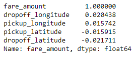
The numbers don’t look very encouraging. Latitudes and longitudes have little to do with fare amounts, at least in their present form. And yet intuitively, they should have a lot do with fare amounts since they specify starting and ending points and longer rides incur higher fares.
Now comes the fun part: creating whole new columns of data that have more impact on the outcome — columns whose values are computed from values in other columns. Add columns specifying the day of the week (0=Monday, 1=Sunday, and so on), the hour of the day that the passenger was picked up (0-23), and the distance (by air, not on the street) in miles that the ride covered. To compute distances, this code assumes that most rides are short and that it is therefore safe to ignore the curvature of the earth.
import datetime
from math import sqrt

for i, row in df.iterrows():
    dt = datetime.datetime.strptime(row['pickup_datetime'], '%Y-%m-%d %H:%M:%S UTC')
    df.at[i, 'day_of_week'] = dt.weekday()
    df.at[i, 'pickup_time'] = dt.hour
    x = (row['dropoff_longitude'] - row['pickup_longitude']) * 54.6 # 1 degree == 54.6 miles
    y = (row['dropoff_latitude'] - row['pickup_latitude']) * 69.0   # 1 degree == 69 miles
    distance = sqrt(x**2 + y**2)
    df.at[i, 'distance'] = distance

df.head()
We no longer need all of those columns, so use these statements to remove the ones that won’t be used:
df.drop(columns=['pickup_datetime', 'pickup_longitude', 'pickup_latitude', 'dropoff_longitude', 'dropoff_latitude'], inplace=True)
df.head()
Let’s check the correlation again:
corr_matrix = df.corr()
corr_matrix["fare_amount"].sort_values(ascending=False)
There still isn’t a strong correlation between distance traveled and fare amount. Perhaps this will explain why:
df.describe()
Here is the output:
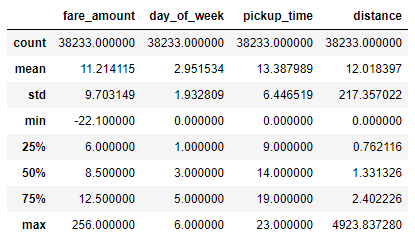
The dataset contains outliers, and outliers frequently skew the results of machine-learning models. Filter the dataset by eliminating negative fare amounts and placing reasonable limits on fares and distance, and then run a correlation again:
df = df[(df['distance'] > 1.0) & (df['distance'] < 10.0)]
df = df[(df['fare_amount'] > 0.0) & (df['fare_amount'] < 50.0)]

corr_matrix = df.corr()
corr_matrix["fare_amount"].sort_values(ascending=False)
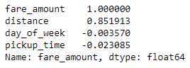
That looks better! The correlation between the day of the week, the hour of day, and fare amount is still weak, but that’s not surprising since distance traveled is the main factor that drives taxi fares. Let’s leave those columns in since it makes sense that it might take longer to get from point A to point B during rush hour, or that traffic at 5:00 p.m. Friday might be different than traffic at 5:00 p.m. on Saturday.
Now it’s time to train a regression model. We’ll try three different regression algorithms to determine which one produces the most accurate results, and use cross-validation to increase confidence in those results. Start by splitting the data for training and testing:
from sklearn.model_selection import train_test_split

x = df.drop(['fare_amount'], axis=1)
y = df['fare_amount']
x_train, x_test, y_train, y_test = train_test_split(x, y, test_size=0.2, random_state=0)
Now train and score a linear-regression model:
from sklearn.linear_model import LinearRegression

model = LinearRegression()
model.fit(x_train, y_train)

model.score(x_test, y_test)
Score the model using 5-fold cross-validation to get a more accurate assessment of its accuracy:
from sklearn.model_selection import cross_val_score

cross_val_score(model, x, y, cv=5).mean()
Train a RandomForestRegressor using the same dataset and see how its accuracy compares. Recall that random-forest models train multiple decision trees on the data and average the results of all the trees to make a prediction.
from sklearn.ensemble import RandomForestRegressor

model = RandomForestRegressor(random_state=0)
model.fit(x_train, y_train)

cross_val_score(model, x, y, cv=5).mean()
Train a third model that uses GradientBoostingRegressor. Gradient-boosting machines use multiple decision trees, each of which is trained to compensate for the error in the output from the previous one.
from sklearn.ensemble import GradientBoostingRegressor

model = GradientBoostingRegressor(random_state=0)
model.fit(x_train, y_train)

cross_val_score(model, x, y, cv=5).mean()
Which model produced the highest cross-validated coefficient of determination?
Finish up by using the trained model to make a pair of predictions. First, estimate what it will cost to hire a taxi for a 2-mile trip at 5:00 p.m. on Friday afternoon:
model.predict([[4, 17, 2.0]])
Now predict the fare amount for a 2-mile trip taken at 5:00 p.m. one day later (on Saturday):
model.predict([[5, 17, 2.0]])
Does the model predict a higher or lower fare amount for the same trip on Saturday afternoon? Does this make sense given that the data comes from New York City cabs?
Get the Code
You can download a Jupyter notebook containing the taxi-fare example from the machine-learning repo that I maintain on GitHub. Feel free to check out the other notebooks in the repo while you’re at it. Also be sure to check back from time to time because I am constantly uploading new samples and updating existing ones.