My previous post introduced two popular algorithms for detecting faces in photographs: Viola-Jones, which relies on machine learning, and MTCNNs, which rely on deep learning. Face detection is a special case of object detection, in which computers detect and identify objects in images. Identifying an object is an image-classification problem, something at which CNNs excel. But finding objects to identify poses a different challenge.
Object detection is challenging because objects aren’t perfectly cropped and aligned as they are in images used for classification tasks. In addition, a scene might contain several objects, in which case each needs to be located before it can be classified. Self-driving cars analyze video frames to identify objects such as cars, traffic lights, and pedestrians. By itself, a CNN trained to do conventional image classification using carefully prepared training images is powerless to help.
Object detection has grown in speed and accuracy in recent years, and state-of-the-art methods rely on deep learning. In particular, they rely on CNNs. Let’s discuss how CNNs do object detection and identification and try our hand at it using a pretrained object-detection model.
R-CNNs
One way to apply deep learning to the task of object detection is to use region-based CNNs, also known as region CNNs or simply R-CNNs. The first R-CNN was introduced in a 2014 paper entitled “Rich feature hierarchies for accurate object detection and semantic segmentation.” The model described in the paper comprises three stages. The first stage scans the image and identifies up to 2,000 bounding boxes representing regions of interest – regions that might contain objects. The second stage is a deep CNN that extracts features from each region of interest. The third is a support-vector machine (SVM) that classifies the features. The output is a collection of bounding boxes with class labels and probabilities. Since each object in the image typically generates multiple overlapping boxes, an algorithm called non-maximum suppression (NMS) filters the output from the SVM and picks the best bounding box for each object detected in the image.
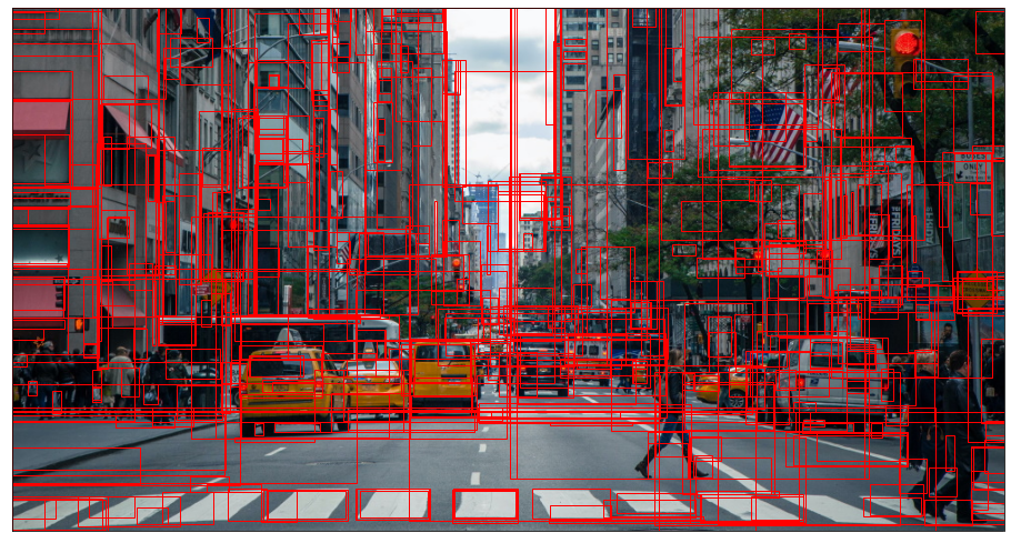
The first stage of most R-CNN implementations uses an algorithm called selective search to identify regions of interest. The illustration below shows the first 500 bounding boxes generated when OpenCV’s implementation of selective search is run over an image. Submitting a targeted list of regions to the CNN is faster than a brute-force sliding-window approach that inputs the contents of the window to the CNN at every stop.
Even with selective search narrowing the list of candidate regions input to stage 2, an R-CNN can’t do object detection in real time. One reason why is that the CNN extracts features not from the image as a whole, but from the 2,000 or so regions of interest identified in stage 1. These regions invariably overlap, so the CNN processes the same pixels multiple times.
A 2015 paper entitled “Fast R-CNN” addressed this by proposing a modified architecture in which selective search or a similar algorithm is first used to identify regions of interest. Then the entire image is passed through the CNN one time, and regions of interest are evaluated using the features extracted from the image. A deep CNN trained on the ImageNet dataset typically serves as the backbone of a Fast R-CNN, but the network is modified to accept two inputs – an image and an array of regions of interest – and produce two outputs: a class prediction for each region, and a regression output containing refined coordinates for the region. Classification is performed by fully connected layers in the network rather than by an SVM, and NMS filters the bounding boxes down to the ones that matter. The result is a system that trains an order of magnitude father than R-CNN, makes predictions two orders of magnitude faster, and is slightly more accurate than R-CNN.
A 2016 paper entitled “Faster R-CNN: Towards Real-Time Object Detection with Region Proposal Networks” boosted performance even more by replacing selective search with a separate CNN specially crafted to identify regions of interest from feature maps. Faster R-CNN implementations can perform 10 times faster than Fast R-CNN and do object detection in near real-time. They are typically more accurate than Fast R-CNNs, too, thanks to a CNN’s superior ability to identify candidate regions.
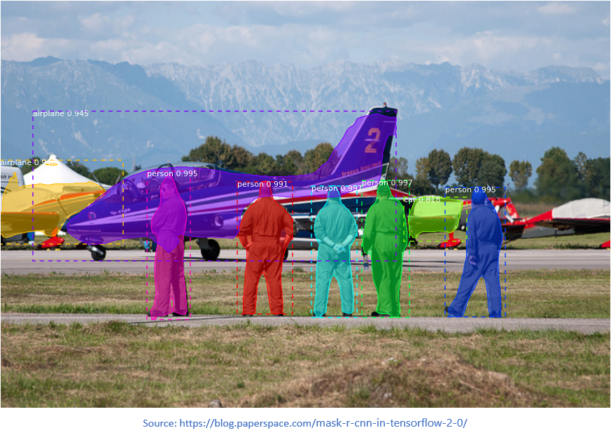
The next chapter in the R-CNN story came in 2017 in a paper entitled “Mask R-CNN.” Mask R-CNNs don’t make Faster R-CNNs faster or more accurate. Rather, they add a feature called instance segmentation that identifies individual pixels comprising an object by generating masks like the ones below. Performance impact is minimal because instance segmentation can be done in parallel with region evaluation. The benefit of Mask R-CNNs is that they provide more detail about the objects they detect. For example, you can tell whether a person’s arms are extended or whether that person is standing up or lying down – something you can’t discern from a simple bounding box.
YOLO
While the R-CNN family of object-detection systems delivers unparalleled accuracy, it leaves something to be desired when it comes to real-time object detection of the type required by, say, self-driving cars. A paper entitled “You Only Look Once: Unified, Real-Time Object Detection” published in 2015 proposed an alternative to R-CNNs known as YOLO that revolutionized the way data scientists think about object detection. From the paper’s introduction:
Humans glance at an image and instantly know what objects are in the image, where they are, and how they interact. The human visual system is fast and accurate, allowing us to perform complex tasks like driving with little conscious thought. Fast, accurate algorithms for object detection would allow computers to drive cars without specialized sensors, enable assistive devices to convey real-time scene information to human users, and unlock the potential for general purpose, responsive robotic systems.
Current detection systems repurpose classifiers to perform detection. To detect an object, these systems take a classifier for that object and evaluate it at various locations and scales in a test image. Systems like deformable parts models (DPM) use a sliding window approach where the classifier is run at evenly spaced locations over the entire image.
More recent approaches like R-CNN use region proposal methods to first generate potential bounding boxes in an image and then run a classifier on these proposed boxes. After classification, post-processing is used to refine the bounding boxes, eliminate duplicate detections, and rescore the boxes based on other objects in the scene. These complex pipelines are slow and hard to optimize because each individual component must be trained separately.
We reframe object detection as a single regression problem, straight from image pixels to bounding box coordinates and class probabilities. Using our system, you only look once (YOLO) at an image to predict what objects are present and where they are.
YOLO systems are characterized by their performance:
Our base network runs at 45 frames per second with no batch processing on a Titan X GPU and a fast version runs at more than 150 fps. This means we can process streaming video in real-time with less than 25 milliseconds of latency. Furthermore, YOLO achieves more than twice the mean average precision of other real-time systems.
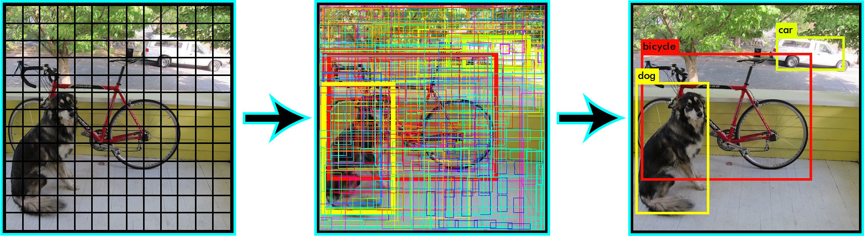
At a high level, YOLO works by dividing an image into a grid of cells and examining each cell for an object. (Think of it as a sliding window in which the windows don’t overlap.) Then it predicts a fixed number of bounding boxes for each cell and assigns class probabilities to the boxes. One CNN handles everything, including feature extraction and regression output designating the sizes and locations of the bounding boxes. At the end, NMS reduces the number of bounding boxes to one per object, and each bounding box is attributed with a class as well as a confidence level – the probability that the box actually contains an object of the specified class.
There are five versions of YOLO referred to as YOLOv1 through YOLOv5. There are also variations such as PP-YOLO and YOLO9000. YOLOv3 processes the image using a 13 x 13 grid, a 26 x 26 grid, and a 52 x 52 grid so it can detect objects large and small (all in one forward pass through the CNN, mind you). It also predicts three bounding boxes per cell and uses a concept called anchor boxes borrowed from Faster R-CNN as a starting point for the bounding boxes. If YOLO has one weakness, it is that it has difficulty detecting small objects that are close together. This is a consequence of the fact that a given cell can only predict one class. More information about YOLO can be found on its creator’s Web site at https://pjreddie.com/darknet/yolo/.
YOLOv3 and Keras
YOLO was originally written using a deep-learning framework called Darknet, but it can be implemented with other deep-learning frameworks, too. The keras-yolo3 project on GitHub contains a Keras implementation of YOLOv3 that can be trained from scratch or initialized with predefined weights and used to make predictions. This version accepts 416 x 416 images. I instantiated the model, initialized it with the weights generated when it was trained on the COCO dataset, and saved it in a Keras H5 file. To simplify usage, I also created a file named yolo3.py containing helper classes and helper functions. It is a modified version of a larger file that’s available in the keras-yolo3 project. I removed elements that weren’t needed for making predictions, rewrote some of the code for improved utility and performance, and added a little of my own, but most of the credit goes to Huynh Ngoc Anh, whose GitHub ID is experiencor. With yolo3.py to lend a hand, you can load YOLOv3 and make predictions with just a few lines of code.
To see YOLOv3 in action, begin by downloading the H5 file containing the trained and serialized model. Name it coco_yolo3.h5 and save it in the directory where your Jupyter notebooks are hosted. (It’s too big for GitHub, so I uploaded it to OneDrive instead.) Then download yolo3.py, abby-lady.jpg, and xian.jpg from my GitHub repo and save them in the same directory.
Next, create a new Jupyter notebook and paste the following code into the first cell:
from yolo3 import *
from keras.models import load_model

model = load_model('coco_yolo3.h5')
model.summary()
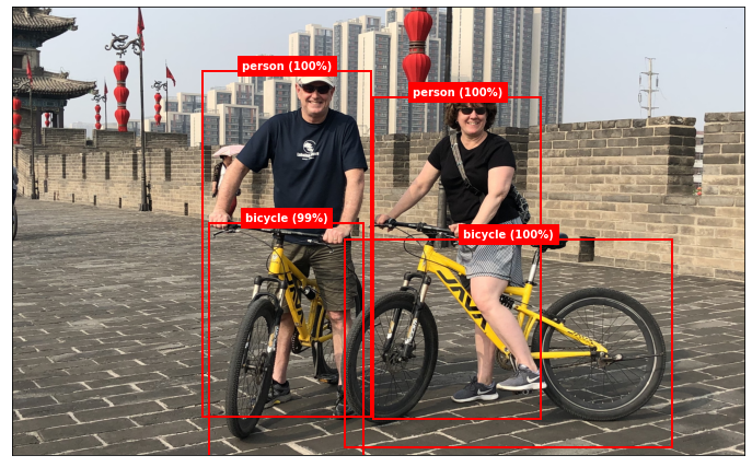
Run the code to import the helper classes and functions in yolo3.py and load the model. Then use the following statements to load a photo of me and my wife biking the city wall surrounding Xian, China:
%matplotlib inline
import matplotlib.pyplot as plt

image = plt.imread('xian.jpg')
width, height = image.shape[1], image.shape[0]
fig, ax = plt.subplots(figsize=(12, 8), subplot_kw={'xticks': [], 'yticks': []})
ax.imshow(image)
Now let’s see if YOLOv3 can detect objects in the image. Use the following code to load the image again, resize it to 416 x 416, preprocess the pixels, and submit the resulting image to the model for prediction:
import numpy as np
from keras.preprocessing.image import load_img
from keras.preprocessing.image import img_to_array

x = load_img('xian.jpg', target_size=(YOLO3.width, YOLO3.height))
x = img_to_array(x) / 255
x = np.expand_dims(x, axis=0)
y = model.predict(x)
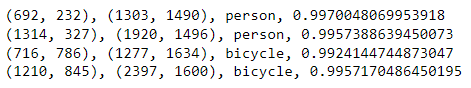
predict returns arrays containing information about objects detected in the image at three resolutions (that is, with grid cells measuring 8, 16, and 32 pixels square), but the arrays need to be decoded into bounding boxes and the boxes filtered with NMS. To help, yolo3.py contains a function called decode_predictions (inspired by Keras’s decode_predictions function) to do all the necessary post-processing. decode_predictions requires the width and height of the original image as input so it can scale the bounding boxes to match the original image dimensions. The return value is a list of BoundingBox objects, each containing the pixel coordinates of a box surrounding an object detected in the scene, along with a label identifying the object and a confidence value from 0.0 to 1.0.
The next step, then, is to pass the predictions returned by predict to decode_predictions and list the bounding boxes:
boxes = decode_predictions(y, width, height)

for box in boxes:
    print(f'({box.xmin}, {box.ymin}), ({box.xmax}, {box.ymax}), {box.label}, {box.score}')
Here’s the output:
The model detected four objects in the image: two people and two bikes. The labels come from the COCO dataset. There are 80 in all, and they’re built into the YOLO3 class in yolo3.py. Use the following command to list them and see all the different types of objects the model can detect:
YOLO3.labels
yolo3.py also contains a helper function named draw_boxes that loads an image from the file system and draws the bounding boxes returned by decode_predictions as well as labels and confidence values. Use the following statement to visualize what the model found in the image:
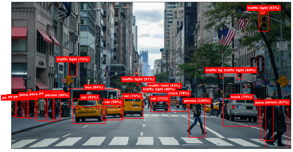
draw_boxes('xian.jpg', boxes)
The output should look like this:
Now let’s try it with another image — this time, a photo of my youngest daughter and the family dog. First show the image and save its width and height:
image = plt.imread('abby-lady.jpg')
width, height = image.shape[1], image.shape[0]
fig, ax = plt.subplots(figsize=(12, 8), subplot_kw={'xticks': [], 'yticks': []})
ax.imshow(image)
Preprocess the image and pass it to the model’s predict method:
x = load_img('abby-lady.jpg', target_size=(YOLO3.width, YOLO3.height))
x = img_to_array(x) / 255
x = np.expand_dims(x, axis=0)
y = model.predict(x)
Show the image again, this time labeled with the objects detected in the image:
boxes = decode_predictions(y, width, height)
draw_boxes('abby-lady.jpg', boxes)
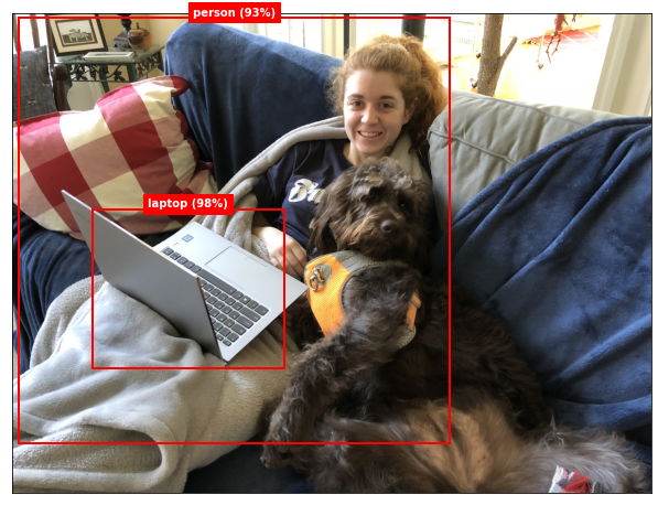
The model detected my daughter and her laptop, but it didn’t detect the dog even though the COCO training images included dogs. Under the hood, it did detect the dog, but with less than 90% confidence. The model’s predict method typically returns information about thousands of bounding boxes, most of which can be ignored because the confidence levels are so low. By default, decode_predictions ignores bounding boxes with confidence scores less than 0.9, but you can override that by including a min_score parameter in the call. Use the following statements to decode the predictions and visualize them again, this time with a minimum confidence level of 55%:
boxes = decode_predictions(y, width, height, min_score=0.55)
draw_boxes('abby-lady.jpg', boxes)
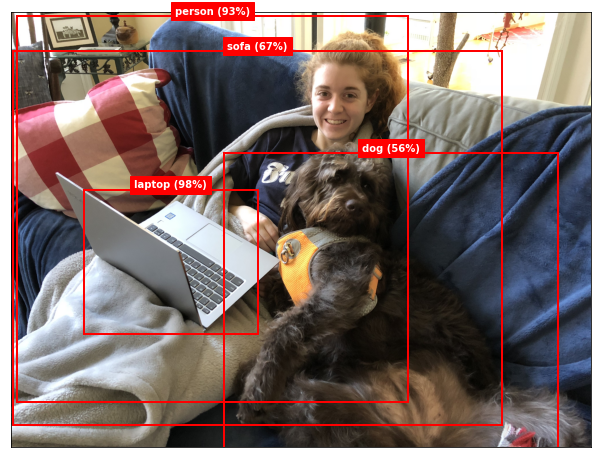
With the confidence threshold lowered to 0.55, the model not only detected the dog, but also the sofa. Because the model was trained on the COCO dataset, it can detect lots of other objects, too, including traffic lights, stop signs, various types of food and animals, and even bottles and wine glasses.
Count People in a Live Webcam Feed
Care to have a little fun? If your computer has a GPU and the GPU version of TensorFlow is installed, run the following code to connect to your webcam and use YOLOv3 to count the number of people in each video frame:
import cv2
import numpy as np
from yolo3 import *
from keras.preprocessing.image import img_to_array
from keras.models import load_model

model = load_model('coco_yolo3.h5')
cam = cv2.VideoCapture(0)

while True:
    # Show the frame
    check, frame = cam.read()
    cv2.imshow('video', frame)

    # Pass the frame to the model and decode the predictions
    x = cv2.cvtColor(frame, cv2.COLOR_BGR2RGB).resize(416, 416)
    x = img_to_array(frame) / 255
    x = np.expand_dims(x, axis=0)
    y = model.predict(x)
    boxes = decode_predictions(y, frame.shape[1], frame.shape[0])

    # Count the number of people in the frame
    count = 0

    for box in boxes:
        if box.label == 'person':
            count += 1

    print(count)

    # Break when the ESC key is pressed
    key = cv2.waitKey(1)
    if key == 27:
        break

cam.release()
cv2.destroyAllWindows()
It can run on CPU, but it’s slow, refreshing just once every few seconds. The count of people in each frame is output with a simple print statement. You could modify my draw_boxes function to accept an image rather than a file name and draw bounding boxes in the video output. Here’s a fun little video in which Joseph Redmon, the creator of YOLO, does just that.
Get the Code
You can download a Jupyter notebook containing object-detection examples from the deep-learning repo that I maintain on GitHub. Feel free to check out the other notebooks in the repo while you’re at it. Also be sure to check back from time to time because I am constantly uploading new samples and updating existing ones.