The three previous posts in this series introduced binary classification and provided working examples of its use, including sentiment analysis and spam filtering. Now it’s time to tackle multiclass classification, in which there are n possible outcomes rather than just two. A great example of multiclass classification is performing optical character recognition: examining a hand-written digit and predicting which digit 0-9 it corresponds to. Another example is looking at a facial photo and identifying the person in the photo by running it through a model trained to recognize hundreds of people.
The great news is that virtually everything you learned about binary classification applies to multiclass classification, too. In Scikit, any classifier that works with binary classification works with multiclass-classification models as well. The importance of this can’t be overstated. Some learning algorithms such as logistic regression only work in binary-classification scenarios. Many machine-learning libraries make you write explicit code to extend logistic regression to perform multiclass classification. Scikit doesn’t. Instead, it makes sure that classifiers such as LogisticRegression work in either scenario, and when necessary, it does extra work behind the scenes to make it happen.
For logistic regression, Scikit uses one of two strategies to extend the algorithm to work in multiclass scenarios. (You can specify which strategy to use with the LogisticRegression class’s multi_class parameter, or accept the default of ‘auto’ and allow Scikit to choose.) One is multinomial logistic regression, which replaces the logistic function with a softmax function that yields multiple probabilities — one per class. The other is one-vs-rest, which trains n binary-classification models, where n is the number of classes that the model can predict. Each of the n models pairs one class against all the other classes, and when the model is asked to make a prediction, it runs the input through all n models and uses the output from the one that yields the highest probability.
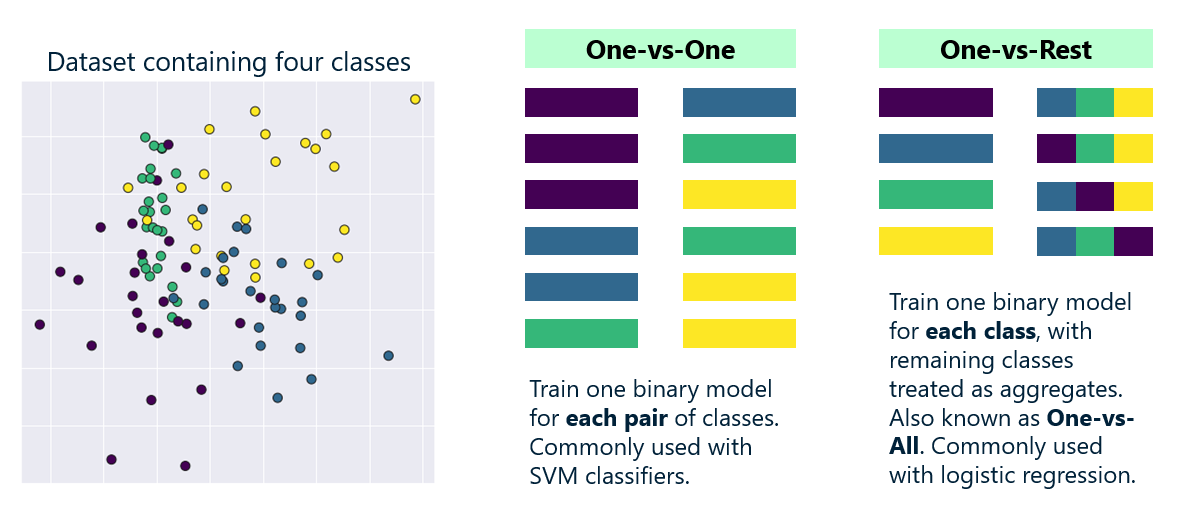
The one-vs-rest approach works well for logistic regression, but for some binary-only classification algorithms, Scikit uses a one-vs-one approach instead. When you use Scikit’s SVC class to perform multiclass classification, for example, Scikit builds one model for each pair of classes. If the model includes four possible classes, Scikit builds no less than seven models under the hood.
You don’t have to know any of this to build a multiclass-classification model. But it does explain why some multiclass-classification models require more memory and train more slowly than others. Some classification algorithms such as random forests and gradient-boosting machines support multiclass classification natively. For algorithms that don’t, Scikit has your back. It fills the gap and does so as transparently as possible.
To reiterate: all Scikit classifiers are capable of performing binary classification and multiclass classification. This simplifies the code you write and lets you focus on building and training models rather than understanding the underlying mechanics of the learning algorithms.
Build a Digit-Recognition Model
Want to experience multiclass classification first-hand? How about a model that examines scanned, hand-written digits and predicts what digits 0-9 they correspond to? The U.S. Postal Service built a similar model many years ago to recognize hand-written zip codes as part of an effort to automate mail sorting. We’ll use a sample dataset that’s built into Scikit: The University of California Irvine’s Optical Recognition of Handwritten Digits dataset, which contains almost 1,800 hand-written digits. Each digit is represented by an 8×8 array of numbers from 0 to 16, with higher numbers indicating darker pixels. We will use logistic regression to make predictions from the data.
Start by creating a Jupyter notebook and executing the following statements in the first cell:
from sklearn import datasets

digits = datasets.load_digits()
print('digits.images: ' + str(digits.images.shape))
print('digits.target: ' + str(digits.target.shape))
Here’s what the first digit looks like in numerical form:
digits.images[0]
And here’s how it looks to the eye:
%matplotlib inline
import matplotlib.pyplot as plt

plt.tick_params(axis='both', which='both', bottom=False, top=False, left=False, right=False, labelbottom=False, labelleft=False)
plt.imshow(digits.images[0], cmap=plt.cm.gray_r)
It’s obviously a 0, but we can confirm that from its label:
digits.target[0]
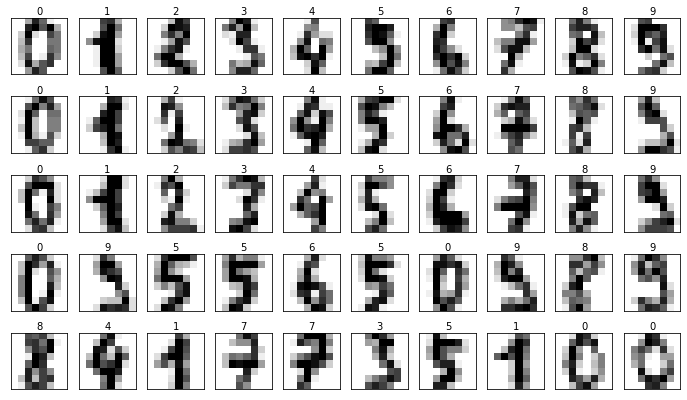
Plot the first 50 images and show the corresponding labels:
fig, axes = plt.subplots(5, 10, figsize=(12, 7), subplot_kw={'xticks': [], 'yticks': []})

for i, ax in enumerate(axes.flat):
    ax.imshow(digits.images[i], cmap=plt.cm.gray_r)
    ax.text(0.45, 1.05, str(digits.target[i]), transform=ax.transAxes)
Classification models work best with balanced datasets. Plot the distribution of the samples:
plt.xticks([])
plt.hist(digits.target, rwidth=0.9)
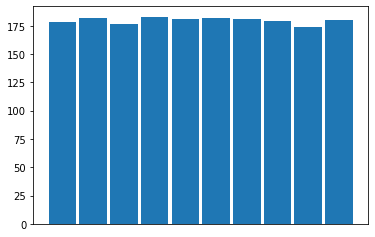
The dataset is pretty well balanced, so let’s split the data and train a logistic-regression model:
from sklearn.linear_model import LogisticRegression
from sklearn.model_selection import train_test_split

x_train, x_test, y_train, y_test = train_test_split(digits.data, digits.target, test_size=0.2, random_state=0)

model = LogisticRegression(max_iter=5000)
model.fit(x_train, y_train)
Use the score method to quantify the model’s accuracy:
model.score(x_test, y_test)
Use a confusion matrix to see how the model performs on the test dataset:
from sklearn.metrics import confusion_matrix

confusion_matrix(y_test, y_predicted)
Pick one of the digits from the dataset and plot it to see what it looks like:
plt.tick_params(axis='both', which='both', bottom=False, top=False, left=False, right=False, labelbottom=False, labelleft=False)
plt.imshow(digits.images[100], cmap=plt.cm.gray_r)
Pass it to the model and see what digit the model predicts it is:
model.predict([digits.data[100]])[0]
What probabilities does the model predict for each possible digit?
model.predict_proba([digits.data[100]])
What is the probability that the digit is a 4?
model.predict_proba([digits.data[100]])[0][4]
When used for binary classification, predict_proba returns two probabilities: one for the negative class (0), and one for the positive class (1). For multiclass classification, predict_proba returns probabilities for each possible class. This permits you to assess the model’s confidence in the prediction returned by predict. Not surprisingly, predict returns the class assigned the highest probability.
Get the Code
You can download a Jupyter notebook containing the digit-classification example from the machine-learning repo that I maintain on GitHub. Feel free to check out the other notebooks in the repo while you’re at it. Also be sure to check back from time to time because I am constantly uploading new samples and updating existing ones.