My previous post demonstrated how to use transfer learning with a CNN trained on millions of facial images to build a facial-recognition model that is remarkably adept at identifying faces. The images used to train the model were carefully cropped so that faces were consistently sized and positioned in the frame.
Suppose you wanted to use that model to tag people in photos uploaded to a Web site. Before submitting faces to the model for identification, you first need to find the faces in the photos, a process known as face detection. Detecting faces like the ones in the photo below isn’t trivial, but it’s a necessary component of an end-to-end facial-recognition system.

This post introduces two widely used algorithms for face detection – one that relies on machine learning, and another that uses deep learning – as well as libraries that implement them. At the end, I’ll present an easy-to-use function that you can call to extract all the facial images from a photo and save them to disk or submit them to a facial-recognition model.
Face Detection with Viola-Jones
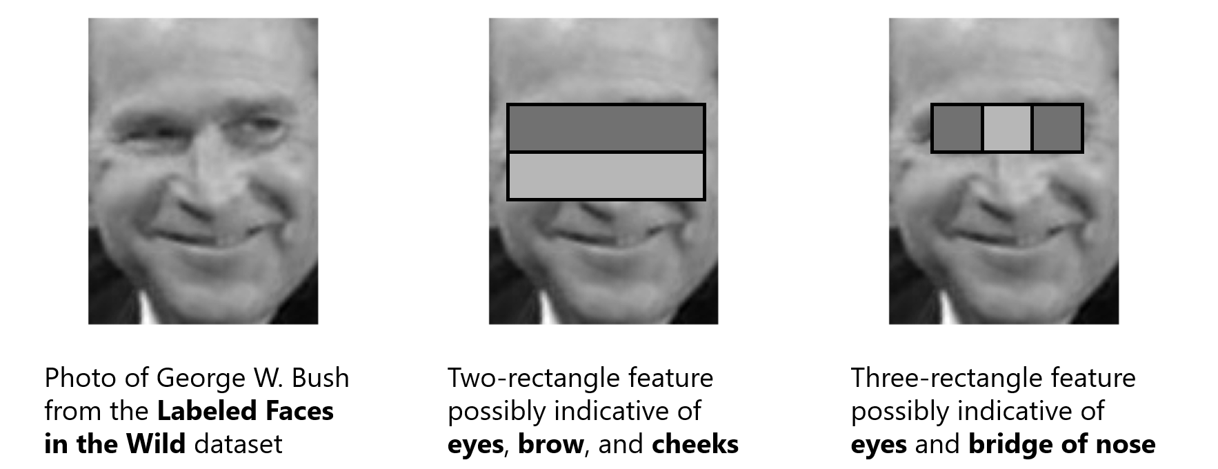
One of the fastest and most popular algorithms for detecting faces in photos stems from a paper published in 2001 entitled “Rapid Object Detection using a Boosted Cascade of Simple Features.” Sometimes known as Viola-Jones (the authors of the paper), the algorithm keys on the relative intensities of adjacent blocks of pixels. For example, the average pixel intensity in a rectangle around the eyes is typically darker than the average pixel intensity in a rectangle immediately below. Similarly, the bridge of the nose is usually lighter than the region around the eyes, so two dark rectangles with a bright rectangle in the middle might represent two eyes and a nose. The presence of many such Haar-like features in a frame at the right locations is a strong indicator that the frame contains a face.
Viola-Jones works by sliding a window over an image looking for frames with Haar-like features in the right places. At each stop, the pixels in the window are scaled to a specified size (typically 24×24), and features are extracted and fed into a binary classifier that either returns positive indicating the frame contains a face or negative indicating it does not. Then the window slides to the next location and the detection regimen begins again.
The key to Viola-Jones’ performance is the binary classifier. A frame that is 24 pixels wide and 24 pixels high contains more than 160,000 combinations of rectangles representing potential Haar-like features. Rather than compute values for every combination, Viola-Jones computes only those that the classifier requires. Furthermore, how many features the classifier requires depends on the content of the frame. The classifier comprises multiple binary classifiers arranged in stages. The first stage might require just one feature. The second stage might require 10, the third might require 20, and so on. Features are only extracted and passed to stage n if stage n-1 returns positive, giving rise to the term cascade classifier.
The diagram below shows a 3-stage cascade classifier. Each stage is carefully tuned to achieve a 100% detection rate using a limited number of features even if the false-positive rate is high. In the first stage, one feature determines whether the frame contains a face. A positive response means the frame might contain a face; a negative response means that it most certainly doesn’t, in which case no further checks are performed. If stage 1 returns positive, however, more features are extracted and passed to stage 2. A frame is only judged to contain a face if all stages return positive, yielding a cumulative false-positive rate near zero. It’s a classic example of combining several weak classifiers to form a strong classifier, a concept introduced in my post on regression algorithms.
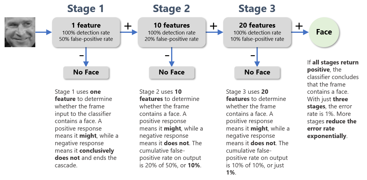
One benefit of this architecture is that frames lacking faces tend to fall out fast because they evoke a negative response early in the cascade. Because most frames don’t contain faces, the algorithm runs very quickly until it encounters a frame that does. In testing with a 38-stage classifier trained on 6,061 features from 4,916 facial images, Viola and Jones found that on average, just 10 features were extracted from each frame.
The efficacy of Viola-Jones depends on the cascade classifier, which is a machine-learning model trained with facial and non-facial images. Training is slow, but predictions are fast. In some respects, Viola-Jones acts like a CNN hand-crafted to extract the minimum number of features needed to determine whether a frame contains a face. To speed feature extraction, Viola-Jones uses a clever mathematical trick called integral images to rapidly compute the difference in intensity between two blocks of pixels. The result is a system that can identify bounding boxes surrounding faces in an image with a relatively high degree of accuracy, and can do so quickly enough to detect faces in live video frames.
OpenCV is a popular computer-vision library. It provides an implementation of Viola-Jones in its CascadeClassifier class, along with an XML file containing a cascade classifier trained to detect faces. The following statements use CascadeClassifier to detect faces in an image and draw rectangles around the faces:
import cv2
from cv2 import CascadeClassifier
import matplotlib.pyplot as plt
from matplotlib.patches import Rectangle
%matplotlib inline

image = plt.imread('PATH_TO_IMAGE_FILE')
fig, ax = plt.subplots(figsize=(12, 8), subplot_kw={'xticks': [], 'yticks': []})
ax.imshow(image)

model = CascadeClassifier(cv2.data.haarcascades + 'haarcascade_frontalface_default.xml')
faces = model.detectMultiScale(image)

for face in faces:
    x, y, w, h = face
    rect = Rectangle((x, y), w, h, color='red', fill=False, lw=2)
    ax.add_patch(rect)
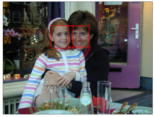
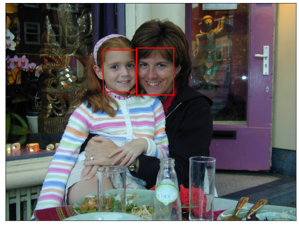
Here’s the output with a photo of my wife and youngest daughter taken in Amsterdam a few years ago:

CascadeClassifier detected the two faces in the photo, but it also suffered a number of false positives. One way to mitigate that is to use the minNeighbors parameter. It defaults to 3, but higher values make CascadeClassifier more selective. With minNeighbors=20, detectMultiScale finds just the faces of my wife and daughter:
faces = model.detectMultiScale(image, minNeighbors=20)
CascadeClassifier frequently requires tuning in this manner to strike the right balance between finding too many faces and finding too few. With that in mind, it is among the fastest face-detection algorithms in existence. It can also be used to detect objects other than faces by loading XML files containing other pretrained classifiers. Here’s a list of XML files included with OpenCV that detect objects using Haar-like features, as well as a list of XML files that detect objects using a different type of discriminator called local binary patterns.
Face Detection with Convolutional Neural Networks
While more computationally expensive, deep-learning methods often do a better job of detecting faces in images than Viola-Jones. In particular, multitask cascaded convolutional neural networks, or MTCNNs, have proven adept at face detection in a variety of benchmarks. They also identify facial landmarks such as the eyes, the nose, and the mouth.
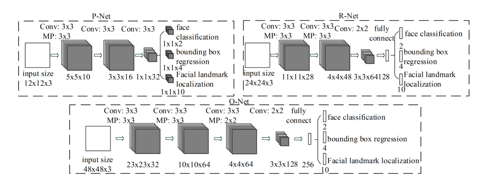
The diagram below comes from the 2016 paper entitled “Joint Face Detection and Alignment Using Multitask Cascaded Convolutional Networks” that proposed MTCNNs. An MTCNN uses three CNNs arranged in series to detect faces. The first CNN, called the Proposal Network, or P-Net, searches the image at various resolutions looking for features that might be indicative of faces. Rectangles identified by P-Net are combined to form candidate face rectangles and input to the Refine Network, or R-Net, which examines the candidate rectangles more closely and rejects those that lack faces. Finally, the output from R-Net is input to the Output Network (O-Net), which further filters candidate rectangles and identifies facial landmarks in rectangles that make it through the filter. These are multitask CNNs because they’re built to produce three outputs each rather than just one. And they’re cascaded like Viola-Jones classifiers to quickly rule out frames that don’t contain faces.
A handy MTCNN implementation is available in the Python package named MTCNN. The following statements use it to detect faces in the same photo of my wife and daughter featured in the previous example:
import matplotlib.pyplot as plt
from matplotlib.patches import Rectangle
from mtcnn.mtcnn import MTCNN
%matplotlib inline

image = plt.imread('PATH_TO_IMAGE_FILE')
fig, ax = plt.subplots(figsize=(12, 8), subplot_kw={'xticks': [], 'yticks': []})
ax.imshow(image)

detector = MTCNN()
faces = detector.detect_faces(image)

for face in faces:
    x, y, w, h = face['box']
    rect = Rectangle((x, y), w, h, color='red', fill=False, lw=2)
    ax.add_patch(rect)
Here’s the result:

MTCNN not only detected the faces of my wife and daughter, but also the face of a statue reflected in the door behind them. Here’s what detect_faces actually returned – a list containing three dictionaries, each corresponding to one of the faces in the photo:
[
  {
    'box': [723, 248, 204, 258],
    'confidence': 0.9997798800468445,
    'keypoints': {
      'left_eye': (765, 341),
      'right_eye': (858, 343),
      'nose': (800, 408),
      'mouth_left': (770, 432),
      'mouth_right': (864, 433)
    }
  },
  {
    'box': [538, 258, 183, 232],
    'confidence': 0.9997591376304626,
    'keypoints': {
      'left_eye': (601, 353),
      'right_eye': (685, 344),
      'nose': (662, 394),
      'mouth_left': (614, 433),
      'mouth_right': (689, 424)
    }
  },
  {
    'box': [1099, 84, 40, 41],
    'confidence': 0.8863282203674316,
    'keypoints': {
      'left_eye': (1108, 101),
      'right_eye': (1123, 96),
      'nose': (1116, 102),
      'mouth_left': (1114, 115),
      'mouth_right': (1127, 111)
    }
  }
]
You can eliminate the face in the reflection in either of two ways: by ignoring faces with a confidence level below a certain threshold, or by passing a min_face_size parameter to the MTCNN function to have detect_faces ignore faces smaller than a specified size. Here’s a modified for loop that does the former:
for face in faces:
    if face['confidence'] > 0.9:
        x, y, w, h = face['box']
        rect = Rectangle((x, y), w, h, color='red', fill=False, lw=2)
        ax.add_patch(rect)
And here’s the result:
The photo at the top of this post was generated with MTCNN using its default settings – that is, without any filtering based on confidence levels or face sizes. Generally speaking, it does a better job out of the box than CascadeClassifier at detecting faces.
Extracting Faces from Photos
Once you know how to find faces in photos, it’s a simple matter to extract facial images so you can use them to train a model or submit them to a model for identification. Here’s a Python function that accepts a path to an image file and returns a list of facial images. By default, facial images are cropped so they’re square (perfect for passing them to a CNN), but you can turn cropping off by passing crop=False:
import numpy as np
from PIL import Image, ImageOps
from mtcnn.mtcnn import MTCNN

def extract_faces(input_file, min_confidence=0.9, crop=True):
    # Load the image
    pil_image = Image.open(input_file)
    pil_image = ImageOps.exif_transpose(pil_image)
    image = np.array(pil_image)

    # Find the faces in the image
    detector = MTCNN()
    faces = detector.detect_faces(image)
    faces = [face for face in faces if face['confidence'] >= min_confidence]
    results = []

    for face in faces:
        x1, y1, w, h = face['box']

        if (crop):
            # Compute crop coordinates
            if w > h:
                x1 = x1 + ((w - h) // 2)
                w = h
            elif h > w:
                y1 = y1 + ((h - w) // 2)
                h = w

        # Extract the facial image and add it to the list
        x2 = x1 + w
        y2 = y1 + h
        results.append(Image.fromarray(image[y1:y2, x1:x2]))

    # Return all the facial images
    return results
I passed the following photo to the function and it returned the faces below:

The items returned from extract_faces are Python Imaging Library (PIL) images, so you can resize them or save them to disk with a single line of code. Here’s a code snippet that extracts all the faces from a photo, resizes them to 224 x 224 pixels, and saves the resized images:
faces = extract_faces('PATH_TO_IMAGE_FILE')

for i, face in enumerate(faces):
    face.resize((224, 224)).save(f'face{i}.jpg')
With extract_faces to help out, it’s a relatively simple matter to generate a set of facial images for training a CNN from a batch of photos on your hard disk, or to extract faces from a photo and submit them to a CNN for identification.
Get the Code
You can download a Jupyter notebook containing face-detection examples from the deep-learning repo that I maintain on GitHub. Feel free to check out the other notebooks in the repo while you’re at it. Also be sure to check back from time to time because I am constantly uploading new samples and updating existing ones.