Building Neural Networks with Keras and TensorFlow

Machine learning isn’t hard when you have a properly engineered dataset to work with. The reason it’s not hard is libraries such as Scikit-learn and ML.NET, which reduce complex mathematical manipulations to a few lines of code. Deep learning isn’t hard, either, thanks to libraries such as the Microsoft Cognitive Toolkit (CNTK), Theano, and PyTorch. But the library that most of the world has settled on for building neural networks is TensorFlow, an open-source framework created by Google that was released under the Apache License 2.0 in 2015.

TensorFlow isn’t limited to building neural networks. It is a framework for performing fast mathematical operations at scale using tensors, which are simply arrays. Tensors can represent scalar values (0-dimensional tensors), vectors (1D tensors), matrices (2D tensors), and so on. A neural network is basically a workflow for transforming tensors. The 3-layer perceptron featured in my previous post takes a 1D tensor containing two values as input, transforms it into a 1D tensor containing three values, and produces a 0D tensor as output. TensorFlow lets you define directed graphs that in turn define how tensors are computed. And unlike Scikit, it supports GPUs.

The learning curve for TensorFlow is rather steep. Another library named Keras provides a simplified Python interface to TensorFlow and has emerged as the Scikit of deep learning. Keras is all about neural networks. Any Keras code that you write ultimately executes in TensorFlow. (Keras can also use CNTK and Theano as back ends, but development has been halted on those frameworks and they are rarely used on new projects.) Keras began life as a separate project in 2015 but was merged into TensorFlow in 2019. Even Google recommends using the Keras API.

Keras offers two APIs: a sequential API and a functional API. The former is simpler and is sufficient for most neural networks. The latter is useful in more advanced scenarios such as networks featuring non-sequential topologies or shared layers. We’ll use the sequential API for our models. If curiosity compels you to learn more about the functional API, I’d suggest that you read How to Use the Keras Functional API for Deep Learning by Jason Brownlee, who is a prolific blogger and one of my favorite authors on machine learning.

If you’re new to neural networks and haven’t read my previous post explaining their mechanics, I highly recommend that you read it before going further.

Building Neural Networks with Keras

Creating a neural network using Keras’s sequential API is simple. You first create an instance of the Sequential class. Then you call add on the Sequential object to add layers. The layers themselves are instances of classes such as Dense, which represents a fully connected layer with a specified number of neurons utilizing a specified activation function. The following statements create the 3-layer network diagrammed in my previous post:

from keras.models import Sequential
from keras.layers import Dense

model = Sequential()
model.add(Dense(3, activation='relu', input_dim=2))
model.add(Dense(1))

This network contains an input layer with two neurons, a hidden layer with three neurons, and an output layer with one neuron. Values passed from the hidden layer to the output layer are transformed by the rectified linear units (ReLU) activation function, which, you’ll recall, adds non-linearity by turning negative numbers into 0s. Observe that you don’t have to add the input layer explicitly. The input_dim=2 parameter in the first hidden layer implicitly creates an input layer with two neurons.

Once all the layers are added, the next step is to call compile. This method doesn’t compile anything in the traditional sense. It simply specifies important attributes such as which optimizer and loss function to use during training. Here’s an example:

model.compile(optimizer='adam', loss='mae', metrics=['mae'])

Let’s walk through the parameters one at a time:

• optimizer=’adam’ tells Keras to use the Adam optimizer to adjust weights and biases in each backpropagation pass during training. Adam is one of eight optimizers that are built into Keras, and it is among the most advanced. It uses an adaptive learning rate and it is always the one I start with in the absence of a compelling reason to do otherwise.
• loss=’mae’ tells Keras to use mean absolute error (MAE) to measure loss. This is appropriate for neural networks intended to solve regression problems.
• metrics=[‘mae’] tells Keras to capture MAE values as the network is trained. This information is used after training is complete to judge the efficacy of the training. You’ll see how in a moment.

Once the network is “compiled,” you train it by calling fit:

hist = model.fit(x, y, epochs=100, batch_size=100, validation_split=0.2)

The fit method accepts many parameters. Here are the ones used in this example:

• x is the dataset’s feature columns
• y is the dataset’s label column – the one containing the values the network will attempt to predict
• epochs=100 tells Keras to train the network for 100 iterations, or epochs. In each epoch, all of the training data passes through the network one time.
• batch_size=100 tells Keras to pass 100 training samples through the network before making a backpropagation pass to adjust the weights and biases. Training takes less time if the batch size is large, but accuracy could suffer. You typically experiment with different batch sizes to find the right balance between training time and accuracy. Do not assume that lowering the batch size will improve accuracy. It frequently does, but sometimes does not.
• validation_split=0.2 tells Keras that in each epoch, it should train with 80% of the rows in the dataset and test, or validate, the network’s accuracy with the remaining 20%. If you’d prefer, you can split the dataset yourself and use the validation_data parameter to pass the validation data to fit. Keras doesn’t offer a function for splitting a dataset, but you can use Scikit’s train_test_split function to do it. One difference between train_test_split and validation_split is that the former splits the data randomly and includes an option for performing a stratified split. validation_split, by contrast, simply splits the dataset into two partitions and does not attempt to stratify.

It might surprise you that if you train the same network on the same dataset several times, the results will be different each time. By default, weights are initialized with random values, and different starting points produce different outcomes. Additional randomness baked into the training process means the network will train differently even if it’s initialized with the same random weights. Rather than fight it, data scientists learn to “embrace the randomness.” If you work the tutorial in the next section, your results will differ from mine. They shouldn’t differ by a lot, but they will differ.

fit returns a history object containing training and validation MAE for each epoch. Charting this data lets you determine whether you trained for the right number of epochs. It also lets you know if the network is underfitting or overfitting. Here’s an example that charts MAE over the course of 100 training epochs:

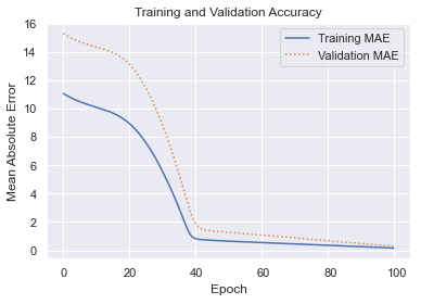
The blue curve reveals how the network fit to the training data. The orange curve shows how it tested against the validation data. Most of the learning was done in the first 40 epochs, but MAE continued to drop as training progressed. The validation MAE matched the training MAE at the end, which is an indication that the network isn’t overfitting. You typically don’t care how well the network fits to the training data. You care about the fit to the validation data, because that indicates how the network performs with data it hasn’t seen before. The greater the gap between the training and validation accuracy, the more network is overfitting.

Once a neural network is trained, you call its predict method to make a prediction:

prediction = model.predict(np.array([[2, 2]]))

In this example, the network accepts two floating-point values as input and returns a single floating-point value as output. The value returned by predict is that output.

Sizing a Neural Network

A neural network is characterized by the number of layers (the depth of the network), the number of neurons in each layer (the widths of the layers), the types of layers (in this example, Dense layers of fully connected neurons), and the activation functions used. There are other layer types, some of which I will introduce in future bog posts. Dropout layers, for example, can increase a network’s ability to generalize by randomly dropping connections between layers during training, while Conv2D layers enable us to build convolutional neural networks (CNNs) that excel at image processing.

When designing a network, how do you pick the right number of layers and the right number of neurons for each layer? The short answer is that the “right” width and depth depends on the problem you’re trying to solve, the dataset you’re training with, and the accuracy you desire. As a rule, you want the minimum width and depth required to achieve that accuracy, and you get there using a combination of intuition and experimentation. That said, here are a few guidelines to keep in mind:

• Greater widths and depths give the network more capacity to “learn” by fitting more tightly to the training data. They also increase the likelihood of overfitting. It’s the validation results that matter, and sometimes loosening the fit to the training data allows the network to generalize better. The simplest way to loosen the fit is to reduce the number of neurons.
• Generally speaking, you prefer greater width to greater depth to avoid the vanishing gradient problem, which diminishes the impact of added layers. The ReLU activation function provides some protection against vanishing gradients, but that protection isn’t absolute. For an explanation, see How to Fix the Vanishing Gradients Problem Using the ReLU.
• Fewer neurons mean less training time. State-of-the-art neural networks trained with large datasets sometime take weeks to train on high-end GPUs, so training time is a big deal.

In real life, data scientists experiment with various widths and depths to find the right balance between training time, accuracy, and the network’s ability to generalize. For a multilayer perceptron, you rarely ever need more than two hidden layers, and one is often sufficient. A network with one or two hidden layers has the capacity to solve even complex non-linear problems. Two layers with 128 neurons each, for example, gives you 16,384 weights that can be adjusted, plus biases. That’s a lot of fitting power. I frequently start with one or two layers of 512 neurons each and halve the width until the validation accuracy drops below an acceptable threshold.

Use a Neural Network to Predict Taxi Fares

Let’s put this knowledge to work building and training a neural network. The problem that we’ll solve is the same one presented in my post on regression modeling: using data from the New York City Taxi & Limousine Commission to predict taxi fares. We’ll use a neural network as a regression model to make the predictions.

To work the following tutorial, you will need to install Keras and TensorFlow if they aren’t installed already. Installing the latest version of TensorFlow installs Keras, too. You can do a pip install or install into environments such as Anaconda. Additional setup is required to enable GPU support.

Download the CSV file containing the dataset and copy it into the directory where your Jupyter notebooks are hosted. Then use the code below to load the dataset. It contains about 55,000 rows and is a subset of a much larger dataset that was recently used in Kaggle’s New York City Taxi Fare Prediction competition:

import pandas as pd
import matplotlib.pyplot as plt
%matplotlib inline
import seaborn as sns
sns.set()
 
df = pd.read_csv('taxi-fares.csv')
df.head()

The data requires a fair amount of prep work before it’s useful — something that is not uncommon in machine learning. Use the following statements to transform the raw dataset into one suitable for training:

import datetime
from math import sqrt

df = df[df['passenger_count'] == 1]
df = df.drop(['key', 'passenger_count'], axis=1)

for i, row in df.iterrows():
    dt = datetime.datetime.strptime(row['pickup_datetime'], '%Y-%m-%d %H:%M:%S UTC')
    df.at[i, 'day_of_week'] = dt.weekday()
    df.at[i, 'pickup_time'] = dt.hour
    x = (row['dropoff_longitude'] - row['pickup_longitude']) * 54.6
    y = (row['dropoff_latitude'] - row['pickup_latitude']) * 69.0
    distance = sqrt(x**2 + y**2)
    df.at[i, 'distance'] = distance

df.drop(['pickup_datetime', 'pickup_longitude', 'pickup_latitude', 'dropoff_longitude', 'dropoff_latitude'], axis=1, inplace=True)

df = df[(df['distance'] > 1.0) & (df['distance'] < 10.0)]
df = df[(df['fare_amount'] > 0.0) & (df['fare_amount'] < 50.0)]
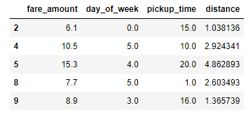
df.head()

The resulting dataset contains columns for the day of the week (0-6, where 0 corresponds to Monday), the hour of day (0-23), and the distance traveled in miles, and from which outliers have been removed:

The next step is to create the neural network. Use the following statements to create a network with an input layer that accepts three values (day, time, and distance), two hidden layers with 512 neurons each, and an output layer with a single neuron (the predicted fare amount):

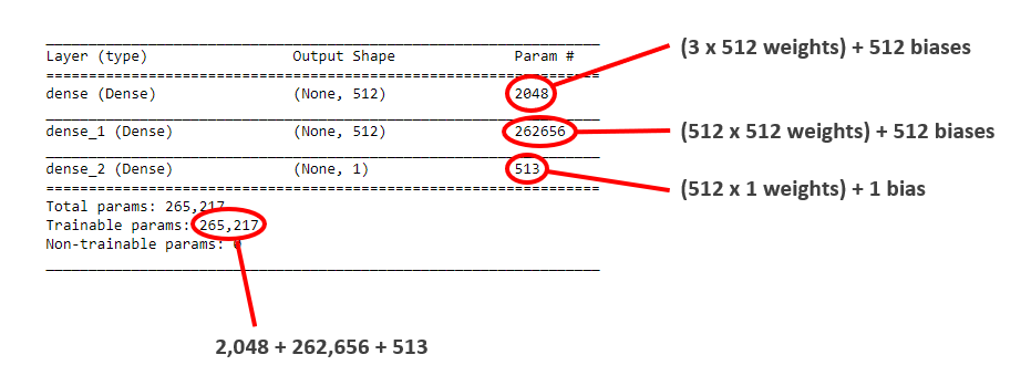
from keras.models import Sequential
from keras.layers import Dense

model = Sequential()
model.add(Dense(512, activation='relu', input_dim=3))
model.add(Dense(512, activation='relu'))
model.add(Dense(1))
model.compile(optimizer='adam', loss='mae', metrics=['mae'])
model.summary()

The call to summary in the last statement produces a concise summary of the network topology, including the number of trainable parameters – weights and biases that can be adjusted to fit the network to a dataset. For a given layer, the parameter count is the product of the number of neurons in that layer and the previous layer (the number of weights connecting the neurons in the two layers) plus the number of neurons in the layer (the biases associated with those neurons). This network is a relatively simple one, and yet it features more than a quarter million knobs and dials that can be adjusted to fit it to a dataset.

Now separate the feature columns from the label column and use them to train the network. Set validation_split to 0.2 to validate the network using 20% of the training data. Train for 100 epochs and use a batch size of 100. Given that the dataset contains more than 38,000 samples, this means that about 380 backpropagation passes will be performed in each epoch:

x = df.drop('fare_amount', axis=1)
y = df['fare_amount']

hist = model.fit(x, y, validation_split=0.2, epochs=100, batch_size=100)

Use the history object returned by fit to plot the training and validation accuracy for each epoch:

err = hist.history['mae']
val_err = hist.history['val_mae']
epochs = range(1, len(err) + 1)

plt.plot(epochs, err, '-', label='Training MAE')
plt.plot(epochs, val_err, ':', label='Validation MAE')
plt.title('Training and Validation Accuracy')
plt.xlabel('Epoch')
plt.ylabel('Mean Absolute Error')
plt.legend(loc='upper right')
plt.plot()

Your results will be slightly different than mine, but should look something like this:

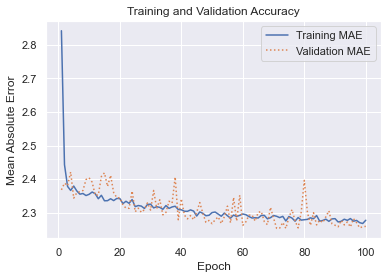
The final validation MAE was about 2.25, which means that on average, a taxi fare predicted by this network should be accurate to within about $2.25.

Recall from my post on regression modeling that a common accuracy measure for regression models is the coefficient of determination, or R² score. Keras doesn’t have a function for computing R² scores, but Scikit does. To that end, use the following statements to compute R² for the network:

from sklearn.metrics import r2_score

r2_score(y, model.predict(x))

Again, your results will differ from mine, but will probably land around 0.74 to 0.75.

Finish up by using the model to predict what it will cost to hire a taxi for a 2-mile trip at 5:00 p.m. on Friday afternoon:

import numpy as np

model.predict(np.array([[4, 17, 2.0]]))

Now predict the fare amount for a 2-mile trip taken at 5:00 p.m. one day later (on Saturday):

model.predict(np.array([[5, 17, 2.0]]))

Does the model predict a higher or lower fare amount for the same trip on Saturday afternoon? Do the results make sense given that the data comes from New York City cabs?

Before you close out this notebook, use it as a basis for further experimentation. Here are a few things you can try to gain further insights into neural networks:

• Run the notebook from start to finish a few times and note the differences in R² scores as well as the MAE curves. Remember that neural networks are initialized with random weights each time they’re created, and randomness during the training process further ensures that the results will vary from run to run.
• Vary the width of the hidden layers. I used 512 neurons in each layer and found that doing so produced acceptable results. Would 128, 256, or 1,024 neurons per layer improve the accuracy? Try it and find out. Since the results will vary slightly from one run to the next, it might be useful to train the network several times in each configuration and average the results.
• Vary the batch size. What effect does that have on training time, and why? How about the effect on accuracy?

Finally, try reducing the network to one hidden layer containing just 16 neurons. Train it again and check the R² score. Does the result surprise you? How many trainable parameters does this network contain?

Get the Code

You can download a Jupyter notebook containing the taxi-fare example from the deep-learning repo that I maintain on GitHub. Feel free to check out the other notebooks in the repo while you’re at it. Also be sure to check back from time to time because I am constantly uploading new samples and updating existing ones.